Understanding the Family of Transformer Models. Part IV - Memory
Apr 4, 2022 by Shuo-Fu "Michael" Chen
Memory is the recordings of experiences, knowledge, or skills acquired passively or learned actively. In human neural network, memory consolidation, storage, and retrieval involve different brain regions, dependent upon the type of learning and modality of stimuli.[1][2] There are at least two stages, short-term memory (STM) and long-term memory (LTM), in human memory formation, and consolidation of LTM likely involves interaction of brain systems in reorganizing and stabilizing distributed connections.[2] Consolidated memories, when reactivated during retrieval, return to a labile state that is sensitive to disruption, requiring “reconsolidation” to persist.[57] Influenced by digital computer, human working memory (WM) models contain not only storages but also processes that integrate STM and LTM to plan and carry out behavior.[55][56] In von Neumann computer architecture, the necessity to have a memory organ, separated from central processing organs, to carry out long and complicated sequences of operations has been considered at the onset.[3] On the contrary, in artificial neural networks, especially Transformer-based architectures, model parameters play a mixed roles of both memory and compute (e.g. [4]) and scaling up memory is accompanied with increasingly prohibitive computing cost in either pre-training-centric[5] or fine-tuning-centric[6][7] approaches. To reduce computing cost while maintaining memory scale, strategies of activating only a subset of model parameters for each input example have been developed to achieve comparable or better performance on mixture-of-experts architecture.[8][9][10]
It is worth noting that although memory and storage are interchangeable terms in neuroscience, they are different in modern computers, in which memory refers to volatile random access memory and storage refers to non-volatile hard disk drive and solid-state drive. The usage of the two terms in artificial neural networks follows those in neuroscience, unless otherwise specified.
Before the advent of the Transformer for large-scale language modeling, explicit memory modules have been incorporated into neural networks for various purposes. Long Short-Term Memory (LSTM)[25] recurrent neural network (RNN) uses memory cells and gate units to overcome the vanishing error problem in backpropagation through extended time steps. Neural Turing Machine (NTM)[26] takes inspiration from biological working memory and digital computer design to extend neural network, feedforward or LSTM, with an external memory matrix that has multi-head attentional reading/writing operations. Memory Networks (MN)[27] attempt to rectify RNN’s difficulty in performing memorization, by combining a memory (an array of objects, e.g., vectors or strings) and four components: I (maps input to feature space), G (updates, compresses, and generalizes memories), O (produces output by selecting top matching memories for the input), and R (can be an RNN that maps output to response). End-To-End Memory Networks (MemNN)[28] improves MN by replacing the hard max operations within each layer of MN with a continuous (attention-like) weighting from the softmax so that the MemNN can be trained end-to-end from input-output pairs. Differentiable Neural Computer (DNC)[11] tries to bring the benefits of an addressable memory of a computer to neural networks by providing an LSTM with read-write access to an external memory matrix, which differs from NTM and MN by using differentiable attention mechanisms for memory access. Sparse Access Memory (SAM)[29] tries to resolve the difficulty in training NTM and DNC when memory size is scaled up, by using sparse content-based read and write operations. Dynamic Neural Turing Machine (D-NTM)[30] addresses the limitation of fixed distance between consecutive memory cells in the location-based addressing strategy of NTM, by introducing a learnable address vector for each memory cell of the NTM with least recently used memory addressing mechanism. It showed that discrete, non-differentiable attention mechanism for memory addressing can outperform continuous, differentiable attention mechanism for episodic QA task. Temporal Automatic Relation Discovery in Sequences (TARDIS)[31] tests the hypothesis that memory augmented RNNs can reduce the effects of vanishing gradients by creating shortcut (or wormhole) connections through time to the past to propagate the gradients more effectively. The memory structure of TARDIS is similar to NTM and D-NTM, but its memory read and write operations use discrete addressing. The results show that the wormhole connections can significantly reduce the effects of the vanishing gradients by shortening the paths that the signal needs to travel between the dependencies.
Since the advent of Transformer, various forms of memories have been developed to extend Transformer-based models for lower computational cost and/or better performance on tasks involving long temporal dimension. This article surveys recent studies on Transformer-based architecture for memory-augmented language modeling and memory replay for lifelong language learning.
Memory-Augmented Language Modeling
Understanding a long document with linguistic relations between temporally distant parts has been a challenge for Transformer-based language models, where input lengths are limited. An approach to address the challenge is to extend the attention span beyond input segments by introducing memory modules for past context, as in Transfomer-XL and Compressive Transformer, where the “memory” represents stored hidden states of past tokens or segments. Transfomer-XL and Compressive Transformer have become standard baseline models in recent studies on memory-augmented language modeling. Different approaches of incorporating memory modules into Transformer-based language models have been shown to improve perplexity performance and/or reduce computational cost. These recent studies can be divided into three categories: using external key-value datastore as memory, using special network layer as memory, and using special input tokens as memory.
External Key-Value Datastore as Memory
Using external key-value datastore as memory to augment Transformer-based language models bears some resemblance to retrieval-augmented language models. The external knowledge store used in the latter cannot be referred to as “memory” because (1) they often are not the dataset used for pre-training the language models, but are a dataset for downstream question-answering tasks; (2) they are stored in input embedding space, not in the key space encoded by the learned parameters of the language models being evaluated; (3) they are used more akin to open-book exam, not memory-dependent closed-book exam. Three examples of memory-augmented language models using external key-value datastore are covered here: kNN-LM[13], SPALM[12], and Memorizing Transformer[17]. In kNN-LM and SPALM, the external memory stores are built by a single pass of training dataset through the pre-trained LMs and then fixed afterwards. Memory retrieval is done for inference only in kNN-LM, but for both training and inference in SPALM. In Memorizing Transformer, the external memory is built during training, causing a distributional shift in the keys and values in the external memory early in the training. All the three approaches substantially outperform Transformer-XL of comparable size on long-form text modeling measured in perplexity.
kNN-LM
Khandelwa et al. (2019)[13] introduced \(\mathit{k}\)NN-LM (\(\mathit{k}\)-nearest neighbors language model) that uses a key-value datastore as memory, where keys are encoded context vectors, values are next tokens, and retrieval is based on \(\mathit{k}\)-nearest neighbors to encoded query vectors, to augment pre-trained, decoder-only Transformer-based language models. The write process of the datastore is not a part of the model training or evaluation. The datastore is static after it is built with a pre-trained LM in a separate process. The read (i.e., retrieval) process is used only at the inference time, as illustrated in the Figure below.

Given a context sequence of tokens \(c_t=(w_1,...,w_{t-1})\), an autoregressive LM estimates \(p(w_t|c_t)\), the distribution over the target token \(w_t\). Let \(f(\cdot)\) be the function that maps a context \(c\) to a fixed-length vector representation computed by the pre-trained LM. Then, given the \(i\)-th training example \((c_i,w_i)\in\mathcal{D}\), the key \(k_i\) is defined as the vector representation of the context \(f(c_i)\) and the value \(v_i\) is the target word \(w_i\). The datastore \((\mathcal{K},\mathcal{V})\) is the set of all key-value pairs constructed from all the training examples in \(\mathcal{D}\): \((\mathcal{K},\mathcal{V})=\{(f(c_i),w_i)|(c_i,w_i)\in\mathcal{D}\}\). This can be done with a single forward pass over the training set of the LM, where the representations learned by the LM remain unchanged. At test time, for an input context \(x\), the LM generates (1) the output distribution over next words \(p_{LM}(y|x)\) and (2) the context representation \(f(x)\). The model queries the datastore with \(f(x)\) to retrieve its \(k\)-nearest neighbors \(\mathcal{N}\) according to squared \(L^2\) (Euclidean) distance function \(d(k_i,f(x))\). Then, it computes a distribution over neighbors based on a softmax of their negative distances, while aggregating probability mass for each vocabulary item across all its occurrences in the retrieved targets (items that do not appear in the retrieved targets have zero probability): \(p_{kNN}(y|x)\propto\sum\limits_{(k_i,v_i)\in\mathcal{N}}\mathrm{\mathbb{1}}_{y=v_i}\exp(-d(k_i,f(x)))\). The final \(\mathit{k}\)NN-LM distribution \(p(y|x)\) is a linear interpolation between the nearest neighbor distribution \(p_{kNN}\) and the model distribution \(p_{LM}\) using a tuned parameter \(\lambda\): \(p(y|x)=\lambda p_{kNN}(y|x)+(1-\lambda)p_{LM}(y|x)\).
The datastore contains one entry per target in the training set, which can be up to billions of examples. To speed up search, FAISS library is used, which clusters the keys, looks up neighbors based on the cluster centroids, and stores compressed versions of the vectors. In this study, \(L^2\) distance outperforms inner product distance for FAISS retrieval for \(\mathit{k}\)NN-LM.
Four corpora are used: Wiki-3B, WikiText-103, Wiki-100M from Wikipedia and Toronto Books Corpus, containing 2.87B, 103M, 100M, and 0.7B tokens, respectively. The average number of tokens per Wikipedia article is about 3,625. The average number of words per book is 89,223 in the Book Corpus. A decoder-only Transformers with 16 layers, each with 16 self-attention heads, is used for LM. The context length for (WikiText-103, other three corpora) are (3,072, 1,024), (2,560, 512), and (\(\geqslant\)1,536,\(\geqslant\)512) for training, evaluation, and key-encoding, respectively. The LM is trained to minimize the negative log-likelihood of the training corpus and evaluated by perplexity on held out data. The keys used for \(\mathit{k}\)NN-LM are the 1024-dimensional representations fed to the feedforward network, after self-attention and layernorm, in the final layer of the Transformer LM. A single forward pass is performed over the training set with the trained model in order to save the keys and values. A FAISS index is created using 1M randomly sampled keys to learn 4,096 cluster centroids. Keys are quantized to 64-bytes for efficiency. During inference, the index looks up 32 cluster centroids and 1,024 nearest neighbors are retrieved. The computational cost to generate the datastore in a single pass over the training set amounts to a fraction of the cost of training for one epoch on the same data.
The \(\mathit{k}\)NN-LM substantially outperforms the base LM, the base LM + Transformer-XL, and the base LM + Continuous Cache on WikiText-103. The Continuous Cache is the technique of saving and retrieving neighbors from earlier examples in the \(\mathit{test}\) document. Combining \(\mathit{k}\)NN-LM and Continuous Cache outperforms \(\mathit{k}\)NN-LM, indicating that the two approaches are complementary. On BookCorpus, the \(\mathit{k}\)NN-LM also outperforms the base LM, indicating that the approach works for multiple domains.
Combining the LM trained with Wiki-100M and the datastore built with Wiki-3B significantly outperforms LM trained with Wiki-100M or Wiki-3B without a datastore, suggesting that rather than training LMs on ever larger datasets, a better performing model can be built with a smaller training dataset and augmented with a \(\mathit{k}\)NN datastore built with a larger corpus. The performance of \(\mathit{k}\)NN-LM improves as the amount of the data used for the datastore increases. The tuned values of \(\lambda\) also increases as the datastore size increases, indicating that the model relies more on the kNN component as the size of the datastore increases.
Domain adaptation experiments compare in-domain training (LM trained and evaluated on BooksCorpus), out-of-domain training (LM trained on Wiki-3B and evaluated on BooksCorpus), and out-of-domain \(\mathit{k}\)NN-LM (datastore on BooksCorpus + LM trained on Wiki-3B and evaluated on BooksCorpus). The out-of-domain \(\mathit{k}\)NN-LM substantially outperforms out-of-domain LM, demonstrating that \(\mathit{k}\)NN-LM allows a single model to be useful in multiple domains, by simply adding a datastore per domain, although the improvement does not reach the level of in-domain LM.
Four hyperparameters are introduced for nearest neighbor search. (1) Key Function. Using the input to the final layer’s feedforward network achieved the largest improvement. Also, normalized representations taken immediately after the layer norm perform better. (2) Number of Neighbors per Query. Each query returns the top-\(k\) neighbors. The performance monotonically improves as the value of \(k\) increases. (3) Interpolation Parameter. The optimal \(\lambda\) values are 0.25 and 0.65 for BookCopus LM + BookCorpus Datastore and Wiki-3B LM + BookCorpus Datastore, respectively. (4) Precision of Similarity Function. In FAISS, the nearest neighbor search computes \(L^2\) distances with quantized keys. The perplexity performance was improved by computing squared \(L^2\) distances with full precision keys (e.g., improved from 16.5 to 16.06 on WikiText-103).
Manually examining cases in which \(p_{kNN}\) was significantly better than \(p_{LM}\) reveals that examples where \(\mathit{k}\)NN-LM is most helpful typically contain rare patterns, such as factual knowledge, names, and near-duplicate sentences from the training set. When \(p_{kNN}\) is significantly better than \(p_{LM}\) for a context-target pair, it means that assigning similar representations to train and test instances appears to be an easier problem than implicitly memorizing the next word in model parameters. Training a vanilla Transformer without dropout will eventually result in zero training loss, meaning the model memorizes all training examples, and low generalization. Interpolating such memorizing LM with a normal LM (i.e., trained with dropout) barely improves the perplexity. In contrast, \(\mathit{k}\)NN-LM memorizes all training data while improving generalization. These results might suggest that autoregressive LM weights immediate prior context more than distant past context for predicting the next word, while \(\mathit{k}\)NN similarity score between train and test contexts weights the entire range of context evenly.
This work offers an alternative method for scaling language models, in which relatively small models learn context representations, and a nearest neighbor search acts as a highly expressive classifier.
SPALM
Yogatama et al. (2021)[12] introduced SPALM (SemiPArametric Language Model) that adaptively combines short-term memory and long-term memory with a Transformer to make predictions. SPALM consists of three main components: (i) a large parametric neural network in the form of a transformer to process local context, (ii) a short-term memory to store extended context, and (iii) a non-parametric episodic memory module that stores information from long-term context. These components are integrated in a single architecture with a gating mechanism, as illustrated in the Figure below.
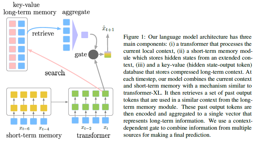
Transformer has limited input sequence length. Instead of considering all previous tokens \(x_{\leq t}\) of a long document, transformer truncates the input to be the most recent \(N\) tokens \(\tilde x_{\leq t}=\{x_{t-N+1},...,x_t\}\) and only operates on this fixed-length window. The extended context of Transformer-XL is used as the short-term memory in this study. Given the current context \(\tilde x_{<t}\), the extended context of length \(M\) is denoted as \(\tilde x_{\leq t-N}=\{x_{t-N-M+1},...,x_{t-N}\}\). The hidden states for \(\tilde x_{\leq t-N}\) are cached and then used as additional states that can be attended to during the forward pass when computing hidden states for the current context \(\tilde x_{\leq t}\), but the values of the states are not updated during the backward pass. Denote \(\mathrm{h}_t^r\), \(\mathrm{H}^r=[\mathrm{h}_{t-N+1}^r,...,\mathrm{h}_t^r]\), and \(\mathrm{E}^r=[\mathrm{SG}(\mathrm{h}_{t-N-M+1}^r),...,\mathrm{SG}(\mathrm{h}_{t-N}^r)]\) as hidden states for token \(x_t\) at layer \(r\), the current (truncated) context \(\tilde x_{\leq t}\), and the extended context \(\tilde x_{\leq t-N}\), respectively, where \(\mathrm{SG}\) is the stop gradient function. \(\mathrm{E}^r\) and \(\mathrm{H}^r\) are concatenated along the length dimension and fed to attention function where each vector is transformed into a query, key, value triplet which are used to produce hidden states, \(\mathrm{H}^{r+1}\), for the next layer.
The long-term memory module is implemented as a key-value database. The key is a vector representation, denoted as \(\mathrm{d}_i\), of a context \(\tilde x_{\leq i}\). Each context is paired with the output token for that context \(x_{i+1}\), which is stored as the value. A key-value entry is stored for each context-token pair in the training corpus, so the number of entries is equal to the number of tokens in the training corpus. A separate vanilla transformer language model is pretrained and its final-layer hidden state is used for \(\mathrm{d}_i\). To predict the next token \(x_{t+1}\) for a given context \(\tilde x_{\leq t}\), the \(\mathrm{d}_t\) is first obtained from the separate pretrained language model. The \(\mathrm{d}_t\) is then used to do a \(k\)-nearest neighbor search on the database to find contexts that are similar to \(\tilde x_{\leq t}\) in the database. The values associated with the top \(k\) such contexts are retrieved from the database as candidate output tokens \(y_1,...,y_K\).
For each \(y_k\), a vector representation \(\mathrm{y}_k\) is created by using the same word embedding matrix that is used in the base model. Then, the information from \(y_1,...,y_K\) are aggregated with a simple attention mechanism using local context \(\mathrm{h}_t^R\) as attention query: \(\mathrm{m}_t=\sum\limits_{k=1}^K\frac{\exp{\mathrm{y}_k}^{\top}\mathrm{h}_t^R}{\sum_{j=1}^K\exp{\mathrm{y}_j}^{\top}\mathrm{h}_t^R}\mathrm{y}_k\). Then a context-dependent gate \(\mathrm{g}_t=\sigma({\mathrm{w}_g}^{\top}\mathrm{h}_t^R)\) that decides how much the model needs to use local information (\(\mathrm{h}_t^R\)) versus long-term information (\(m_t\)) for making the current prediction based on the current context: \(\mathrm{z}_t=(1-\mathrm{g}_t)\odot\mathrm{m}_t+\mathrm{g}_t\odot\mathrm{h}_t^R\) and \(p(x_{t+1}\vert x_{\leq t})=\mathrm{softmax}(\mathrm{z}_t;\mathrm{W})\), where \(\mathrm{w}_g\) is a parameter vector, \(\sigma\) is the sigmoid function, and \(\mathrm{W}\) is the word embedding matrix that is shared for input and output word embeddings. Note that the only additional parameter that needs to be trained is \(\mathrm{w}_g\).
A separate standard transformer language model is first trained and used to generate key (\(\mathrm{d}_i\)) for the database. The key representations are not updated when training the overall model. On the other hand, the value encoder is updated during training since the word embedding matrix is used to represent \(\mathrm{y}_k\). \(k\)-nearest neighbors search is done using ScaNN method for efficient vector similarity search, which includes search space pruning and quantization for Maximum Inner Product Search. During the evaluation, new tokens from the evaluation data are not stored and the database remains static.
SPALM differs from \(k\)NN-LM on three aspects. (1) \(k\)NN-LM only has long-term memory, but SPALM has long-term and short-term memory. (2) \(k\)NN-LM integrates long-term memory at output level (an ensemble technique) during evaluation time, but SPALM integrates long-term memory at hidden states level during training and evaluation. Integration at hidden states level enables multi-modality integration, which is not possible in output-level integration. (3) \(k\)NN-LM uses a fixed interpolation weight \(\lambda\) for all tokens, but SPALM uses a context-dependent gate \(\mathrm{g}_t\) per token.
Word-level language modeling is first evaluated on WikiText-103 for vanilla Transformer, Transformer-XL, \(k\)NN-LM, and SPALM. All models have 18 layers, 512 hidden dimension, 142M total parameters, and 512 input sequence length. For Transformer-XL, the short-term memory length is set to 512 during training and 512 or 3072 during test. The perplexity results show that Transformer-XL substantially outperforms Transformer and \(k\)NN-LM significantly outperforms Transformer-XL, but SPALM and \(k\)NN-LM are not much different (on the development set, SPALM is marginally better; on the test set, \(k\)NN-LM is marginally better). Further improvement over both SPALM and \(k\)NN-LM can be achieved by interpolating SPALM’s output probability with the \(p_{kNN}\) used by \(k\)NN-LM, indicating that incorporating long-term memory into training and interpolating probabilities at test time have some complementary benefits. Word-level language modeling is further evaluated on approximately ten times larger dataset WMT 2019, containing news articles, using the same set of model hyperparameters. The perplexity results show that SPALM significantly outperforms \(k\)NN-LM, Transformer-XL, and Transformer. Unlike WikiText-103, there is no further improvement interpolating the probabilities of SPALM with \(p_{kNN}\). Also, when the distributions of the dev and test sets can be different (e.g., articles from different months), \(k\)NN-LM that relies on tuning \(\lambda\) on the dev set has larger performance discrepancy between the dev and test sets. Character-level language modeling is evaluated on enwik8 dataset, using 24-layer model, 512 hidden size, 100M parameters, and sequence length of 768. Transformer-XL short-term memory length is 1536 for training and 4096 for evaluation. The bits-per-character results show that SPALM outperforms all other models. Interpolating the probabilities of SPALM with \(p_{kNN}\) does not improve performance.
Inspection of neighbor tokens retrieved from the long-term memory for WMT dataset reveals that retrieved neighbors are generally relevant even when they do not match a target word exactly. Retrieved neighbors on enwik8 dataset reveals that information from the long-term memory helps when completing common words, named entities, and corpus-specific formats. SPALM is generally better than both transformer and transformer-XL for predicting (completing) common phrases and named entities that exist in the training set, especially when they are encountered for the first time and have not appeared in the extended context. In cases when Transformer-XL outperforms SPALM, usually the same word has appeared in the extended context, but its probability in SPALM is smoothed by information from the long-term memory.
Distributions of the values of the gates for tokens in WMT and enwik8 show that the values are concentrated around 1 on enwik8, indicating that the model relies on local context most of the time; but the values on WMT are less concentrated around 1, suggesting that the model uses long term memory more than on enwik8. Thus, the gate in SPALM can learn when the long-term memory is needed. When the number of nearest neighbors on the WikiText-103 development set is varied from 1 to 16, the SPAML perplexity is the best at 4 neighbors.
The biggest limitation of SPALM is the necessity to retrieve neighbors for each training token, which results in time consuming training process.
Memorizing Transformer
Wu et al. (2022)[17] introduced Memorizing Transformer that uses an external memory of key-value pairs of previously seen subsequences and a retrieval mechanism of an approximate \(k\)NN attention over the memory. The architecture of the \(k\)NN-augmented transformer is shown in the Figure below. The core model is a vanilla decoder-only transformer. The input text is tokenized, and the tokens are embedded into vector space. The embedding vectors are passed through a series of transformer layers, each of which does dense self-attention, followed by a feed-forward network (FFN). The decoder-only language model uses a causal attention mask and the token embeddings of the last layer are used to predict the next token. Long documents are split into subsequences of 512 tokens, and each subsequence is used as the input for one training step. Subsequences of a long document are fed into the transformer sequentially, from beginning to end. Transformer-XL style cache is also used, which holds the keys and values from the previous training step. When doing self-attention, the cached keys and values are prepended to the current keys and values, and a sliding-window causal mask is used so that each token has a local context that includes the previous 512 tokens.
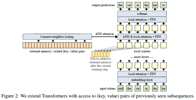
One of the transformer layers near the top of the stack is a \(k\)NN-augmented attention layer, which combines two forms of attention: standard dense self-attention on the local context, which is the input subsequence for the current training step, and an approximate \(k\)NN attention to search into the external memory. The same queries are used for both the local context and the external memory. After each training step, the (key, value) pairs in the local context are appended to the end of the external memory. If the document is very long, old (key, value) pairs will be dropped from the memory to make room for new ones, in a FIFO queue fashion. Thus, for each head, the external memory keeps a cache of the prior \(M\) (key, value) pairs, where \(M\) is the memory size. The \(k\)NN lookup will return a set of retrieved memories, which consist of the top-\(k\) (key, value) pairs that \(k\)NN search returns for each query (i.e., each token) in the input subsequence. As with standard dense attention, an attention matrix is constructed first by computing the dot product of each query against the retrieved keys, then softmax is applied, and finally a weighted sum of the retrieved values is returned. Unlike standard dense attention, the retrieved memories contain a different set of (key, value) pairs for each query.
The results of \(k\)NN-attention and local attention are then combined using a learned gate: \(g=\sigma(b_g)\), \(V_a=V_m\odot g+V_c\odot(1-g)\) where \(\sigma\) is the sigmoid function, and \(\odot\) is element-wise multiplication, \(V_a\) is the combined result of attention, \(V_m\) is the result of attending to external memory, and \(V_c\) is the result of attending to the local context. The bias \(b_g\) is a learned per-head scalar parameter, which allows each head to choose between local and long-range attention. Over time, most heads learned to attend almost exclusively to external memory. For dense attention within the local context, the T5 relative position bias is used. For the retrieved memories, no position bias is used. Multiple long documents of different lengths are packed into a batch, and split into subsequences. Each subsequence in the batch comes from a different document, and thus requires a separate external memory, which is cleared at the start of each new document. The primary difference between Memorizing Transformer and the SPALM above is that the external memory here is gradually filled up during training and continues to be updated during training and testing rather than filled up in a separate process before training and fixed throughout training and testing in SPALM.
During training, as the model moves from early subsequence to later subsequence of a long document, there is a distributional shift in the keys and values that are stored in the external memory. For very large memories, older records may become “stale”. To reduce the effects of staleness, keys and queries are normalized using QKNorm that applies \(\mathcal{l}_2\) normalization to \(Q\) and \(K\) only along the head dimension to make each element of \(QK^{\top}\) the cosine similarity instead of dot product. Normalization does not eliminate staleness, but it ensures that older keys and newer keys do not differ in magnitude. It also helps stabilize training with the Transformer-XL cache. In some experiments, training models from scratch with a large memory sometimes resulted in worse performance than pretraining the model with a small memory of size 8192, and then finetuning it on a larger memory. An approximate \(k\)NN search rather than exact \(k\)NN search is used because it significantly improves the computational speed while achieving a search recall of about 90% of the true top-\(k\).
Five long-form text datasets are used for evaluation: English language books (PG-19), long web articles (C4), technical math papers (arXiv Math), source code (Github), and formal theorems (Isabelle). PG-19 contains full-length books published before 1919, extracted from the Project Gutenberg archive. C4(4K+), the colossal cleaned common crawl, contains documents scraped from the internet and only includes documents \(\geq 4096\) tokens. The arXiv Math dataset contains mathematics papers downloaded from arXiv; the number of tokens per paper is roughly comparable to the number of tokens per book in PG19. Github source code files include languages C, C++, Java, Python, Go, and TypeScript. To capture dependencies between files in a repository, one long document is created for each Github repository by traversing the directory tree and concatenating all of the files within it without specific order. The Isabelle corpus consists of formal mathematical proofs of 684 theories, on topics such as foundational logic, advanced analysis, algebra, or cryptography. All files that make up a theory are concatenated together into one long document in the order according to their import dependencies.
A 12-layer decoder-only transformer is used in this study, with or without Transformer-XL cache, with \(d_{embedding}=1024\), 8 attention heads of \(d=128\), \(d_{\mathrm{FFN}}=4096\). The 9th layer is used as the \(k\)NN-augmented (\(k=32\)) attention layer, unless specified otherwise. A sentence-piece tokenizer is used with a vocabulary size of 32K. To compare models with different context lengths, the number of documents in a batch is adjusted so that there are always \(2^{17}\) tokens in a batch.
Adding external memory to either vanilla Transformer or Transformer-XL improves perplexity across all five datasets by a substantial amount. Increasing the size (up to 65K) of the memory increases the benefit of the memory. For Transformer-XL with context size 2048 and total receptive field of \(2048\times 12\sim25K\), adding an external memory of size 8192 still results in substantial performance gain, suggesting that \(k\)NN attention on memory is more effective than Transformer-XL’s recurrent cache in retrieving information from the distant past. On the other hand, the XL cache provides additional local short-range context at the start of a sequence, which complements the long-range context provided by external memory. Adding a small external memory (size 1536) to a vanilla Transformer performs equally to using local context of size 2048 without external memory, suggesting that lower layers of a Transformer may not need long-range context and having a differentiable memory may not be important. External memory provides a consistent improvement to the model as it is scaled up. The smaller Memorizing Transformer with just 8k tokens in memory can match the perplexity of a larger vanilla Transformer with 5X more trainable parameters.
When using large memories, training was sometimes unstable, possibly due to distributional shift early in the training. Thus, for memories \(\geq 131K\) tokens, the model is first pretrained with a small memory size of 8192 or 65K for 500K steps, and then finetuned with the larger memory for an additional 20K steps. Increasing the size of external memory during finetuning provided consistent gains up to a size of 262K, which is longer than almost all of the documents in arXiv dataset. A Transformer that is pretrained without external memory can be finetuned with an external memory. A pre-trained one billion parameter vanilla Transformer model fine-tuned with external memory quickly learns to use external memory. Within 20K steps (4% of the pre-training time) the fine-tuned model has already closed 85% of the gap between it and the 1B Memorizing Transformer, and after 100k steps it has closed the gap entirely.
Retrieved memories are studied by finding which tokens showed the biggest improvements in cross-entropy loss when the size of the memory was increased and then examining the top-\(k\) retrieved memories for those tokens. The model gained the most when looking up rare words, such as proper names, references, citations, and function names, where the first use of a name is too far away from subsequent uses to fit in the local context. The tokens that contribute to a large improvement in perplexity correspond to sparse memory positions and constitute only a small percentage of total memory. The top-\(k\) retrieved memories for tokens which show the largest improvement in cross-entropy loss show that the model retrieved function and variable names for arXiv math and Github datasets. When predicting the name of a mathematical object or a lemma for the Isabelle corpus, the model looked up the definition from earlier in the proof and found the body of the lemma it needs to predict 6 out of 10 times. This is the first demonstration that attention is capable of looking up definitions and function bodies from a large corpus. The Isabelle case study used a model with two memory layers of size 32K.
Memorizing Transformer is capable of making use of newly defined functions and theorems during test time.
Special Network Layer as Memory
Another category of memory architecture introduces novel memory mechanisms tightly integrated within individual layers of Transformer. Four examples are covered here. (1) Product Key Memory[14] replaces feed-forward sub-layer in 1~3 selected layers of decoder-only Transformer with a memory sub-layer that factorizes attention keys as product sets. (2) Memformer[16] adds a memory reader sub-layer between self-attention sub-layer and feed-forward sub-layer in each layer of the encoder and only one memory writer layer above the encoder stack of the encoder-decoder Transformer. (3) Infinite Memory Transformer[22] adds a different long-term memory at each layer of decoder-only Transformer to store past text sequence’s input embeddings or hidden states. The model uses a set of Gaussian Radial Basis Functions and a multivariate ridge regression to transform a discrete sequence representation into a continuous-space representation and a continuous attention mechanism to obtain long-term memory context representation for a given query. (4) MemSizer[18] replaces self-attention sub-layer in each layer of a decoder-only Transformer with a novel key-value memory layer that uses two adaptor weight matrices to make the attention mechanism scales linearly with input length. The model handles generation steps in a recurrent procedure similar to kernel-based Transformers. Another example, modern Hopfield networks[24] for dense associative memories have been proposed to substitute attention layers of Transformer, but the idea has not been experimented on language modeling task; thus, it is not covered here.
PKM
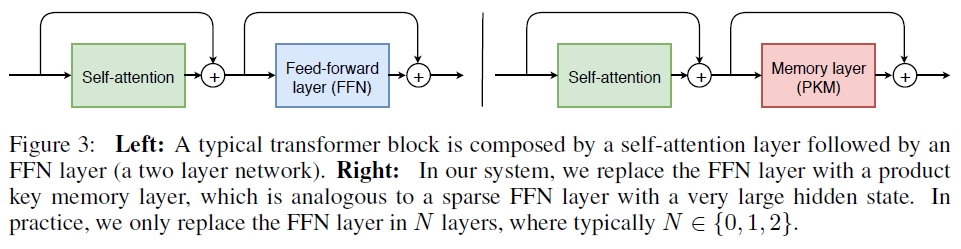
Lample et al. (2019)[14] introduced PKM (Product Key Memory) memory layer that replaces a Feed-forward layer in Transformer architecture, as illustrated in the Figure below. The memory layer is integrated with a residual connection in the network, and the input \(x\) to the memory layer produces \(x+\mathrm{PKM}(x)\) instead of \(x+\mathrm{FFN}(x)\).
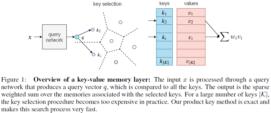
The memory layer is composed of three components: (1) a query network, (2) a key selection module containing two sets of sub-keys, and (3) a value lookup table. The query network \(q\) maps the input \(x\in\mathrm{\mathbb{R}}^d\) to a latent space \(q(x)\in\mathrm{\mathbb{R}}^{d_q}\), where \(q\) is typically a linear mapping or a multi-layer perceptron and \(d_q=512\). A batch normalization layer is added on the top of the query network to help increasing key coverage during training.
In standard key selection and weighting approach, top-\(k\) keys are selected from a set of keys \(\mathcal{K}=\{k_1,...,k_{\vert\mathcal{K}}\vert\}\) by the largest inner product with the query \(q(x)\), where \(k_i\in\mathrm{\mathbb{R}}^{d_q}\). There are three steps: (1) finding the indices of the \(k\) nearest neighbors \(\mathcal{I}=\mathcal{T}_k(q(x)^{\top}k_i)\), where \(\mathcal{T}_k\) denotes the top-\(k\) operator; (2) normalizing the top-\(k\) scores \(w=\mathrm{softmax}((q(x)^{\top}k_i)_{i\in\mathcal{I}})\), where \(w\) is the vector representing normalized scores; and (3) aggregating selected values \(m(x)=\sum_{i\in\mathcal{I}}w_iv_i\), where \(m(x)\) is the resulting memory value vector, as illustrated in the Figure below. All these operations can be implemented using auto-differentiation mechanisms, making the memory layer pluggable in a neural network. The steps (2) and (3) are computationally efficient, to handle only the top-\(k\) keys/values. In contrast, step (1) is not efficient for large memories, for the exhaustive comparison. To circumvent this issue, the product key approach is introduced.
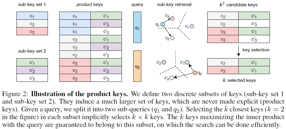
In the product key approach, the query \(q(x)\) is split into two sub-queries \(q_1\in\mathrm{\mathbb{R}}^{d_q/2}\) and \(q_2\in\mathrm{\mathbb{R}}^{d_q/2}\) that are used to find top-\(k\) nearest neighbors in the sub-key (\(\in\mathrm{\mathbb{R}}^{d_q/2}\)) sets \(\mathcal{C}\) and \(\mathcal{C}^{\prime}\), respectively: \(\mathcal{I}_{\mathcal{C}}=\mathcal{T}_k((q_1(x)^{\top}c_i)_{i\in\{1...\vert\mathcal{C}\vert\}})\) and \(\mathcal{I}_{\mathcal{C}^{\prime}}=\mathcal{T}_k((q_2(x)^{\top}c_j^{\prime})_{j\in\{1...\vert\mathcal{C^{\prime}}\vert\}})\). The two sets of selected \(k\) sub-keys are then concatenated in Cartesian product fashion to form \(k^2\) candidate product keys (\(\in\mathrm{\mathbb{R}}^{d_q}\)) that are then used to search for the top-\(k\) product keys nearest to \(q(x)\) in \(\{(c_i,c_j^{\prime})\vert i\in\mathcal{I}_{\mathcal{C}},j\in\mathcal{I}_{\mathcal{C}^{\prime}}\}\). The total number of product keys is \(\vert\mathcal{K}\vert=\vert\mathcal{C}\vert\times\vert\mathcal{C}^{\prime}\vert\), where \(\mathcal{K}=\{(c,c^{\prime})\vert c\in\mathcal{C},c^{\prime}\in\mathcal{C}^{\prime}\}\), as illustrated in the Figure below.
In standard top-\(k\) flat key selection, the complexity is \(\mathcal{O}(\vert\mathcal{K}\times d_q\vert)\), for \(\vert\mathcal{K}\vert\) comparisons of vectors of size \(d_q\). In the two-stage top-\(k\) product key selection, the complexity is \(\mathcal{O}(\sqrt{\vert\mathcal{K}\vert}\times d_q)\) for selecting two sets of top-\(k\) sub-keys and \(\mathcal{O}(k^2\times d_q)\) for selecting top-\(k\) candidate product keys, resulting in the overall complexity \(\mathcal{O}((\sqrt{\vert\mathcal{K}\vert}+k^2)\times d_q)\). Thus, for \(\vert\mathcal{K}\vert=1024^2\) and a small \(k\), selecting top-\(k\) product keys requires about \(10^3\)-fold less operations than selecting top-\(k\) flat keys.
To make the model more expressive, a multi-head memory mechanism is introduced. Each head has its own query network and its own set of sub-keys, but all heads share the same values. As the query networks are independent from each other and randomly initialized, they often map the same input to very different values of the memory. The final multi-head memory value is the sum of the outputs \(m_i(x)\) of each head \(i\): \(m(x)=\sum_{i=1}^H m_i(x)\) where \(H\) is the number of heads. The multi-head memory is different from multi-head attention in that it creates a query per head instead of splitting a query into \(H\) heads.
The Common Craw News corpus is used for this study, which contains about 40M news articles, 28B words, 140GB of data. The validation and test sets are both composed of 5,000 news articles removed from the training set. Byte Pair Encoding (BPE), with 60K BPE splits, is used to reduce the vocabulary size. Three evaluation metrics are used in this study: (1) perplexity on the test set, (2) memory usage defined as the fraction of accessed values during test, and (3) the KL divergence between normalized access weight matrix and uniform distribution. Let \(z^{\prime}\in\mathrm{\mathbb{R}}^{\vert\mathcal{K}\vert}\) be a vector representing access weights to product key memory slots \(z_i^{\prime}=\sum_x w(x)_i\), where \(i\) is the index of a memory slot and \(w(x)\) represents the weights of the keys accessed in the memory when the network is fed with an input \(x\) from the test set (i.e., the \(w(x)\) are sparse with at most \(H\times k\) non-zero elements). Then, \(z=z^{\prime}/ \Vert z^{\prime}\Vert_1\) represents L1-norm-normalized \(z^{\prime}\). The memory usage is \(\frac{\#\{z_i\neq 0\}}{\vert\mathcal{K}\vert}\). The KL divergence is \(\log(\vert\mathcal{K}\vert)+\sum z_i\log(z_i)\), which reflects imbalance in the access patterns to the memory.
The Transformer architecture is decoder only with 16 attention heads and learned positional embeddings. Three layer numbers, 12, 16, or 24 and two hidden dimensions 1024 or 1600 are considered. To retrieve key indices efficiently, the search over sub-keys is performed with FAISS. The memory layers are interspersed at regular intervals; for example, 2 memory layers in 16 layers network are placed at 6th and 12th layers. The main experiments use \(H=4\) memory heads, \(k=32\) keys per head, and \(\vert\mathcal{K}\vert=512^2\) memory slots.
The results show that increasing either the dimensionality or the number of layers leads to significant perplexity improvements in all the models. However, adding a memory layer to the model is more beneficial than increasing the number of layers; adding 2 or 3 memory layers further improves performance. Comparing models with the same number of layers and dimensions, adding memory layers caused small reduction in inference speed for models with 1024 dimensions, but negligible reduction for models with 1600 dimensions. A model with 12 layers and a memory layer obtains better perplexity and almost twice faster than a model with 24 layers and without a memory layer.
Increasing memory size (\(\vert\mathcal{K}\vert\), i.e., \(\vert\mathcal{C}\vert\times\vert\mathcal{C}^{\prime}\vert\)) improves perplexity performance, with inference speed unchanged. Inference speed is mainly affected by the memory usage, which is governed by the number of memory heads and the parameter \(k\), but not the memory size. The batch normalization layer improves the memory usage significantly, along with the perplexity, for large memory sizes (\(\geqslant 147K\)), but it doesn’t help when memory size is small (16K or 65K) where the usage is already close to 100% without batch normalization. When the memory layer replaces the FFN of the layers 4 or 5 in a 6-layer Transformer, the model benefits the most, suggesting that effective use of the memory layer requires operating at higher layer and that it is important to have some layers on top of the memory layer. Increasing the number of memory heads \(h\) or the number of \(k\) for \(k\)-NN improves both the perplexity of the model and the memory usage. Models with identical \(h\times k\) have a similar memory usage and perplexity. Increasing \(h\) or \(k\) also increases computation cost. A good trade-off between performance and speed is \(h=4\) and \(k=32\).
Transformer-based Language models with integrated product key memory layer drastically improve the capacity of the neural network and the perplexity performance with a negligible computational overhead, due to a much better memory usage. Two key ingredients contribute to the efficiency: the factorization of keys as a product set and the sparse read/write access to the memory values.
Memformer
Wu et al. (2020)[16] introduced Memformer that extends encoder-decoder Transformer architecture with a learnable memory system. Given a long document \(x\) that is split into \(T\) segments of length \(L\), each segment \(s_t\) is denoted as \(s_t=[x_{t,1},x_{t,2},...,x_{t,L}]\). The encoder recurrently encodes a segment level memory \(M_t=\mathrm{Encoder}(s_t,M_{t-1})\). The final output of the encoder is fed into the decoder’s cross attention layers to predict the token probabilities of the next segment \(s_{t+1}\) as standard language modeling, \(P(s_t)=\prod\limits_{n=1:L}P_{\mathrm{Decoder}}(x_{t,n}\vert x_{t,<n},M_{t-1})\). The joint probability of the document is defined as the product of each segment’s probability conditioned on all of its previous segments, \(P(x)=\prod\limits_{t=1:T}P_{\mathrm{Model}}(s_t\vert s_{<t})\). Given a text segment as the input, the model can generate the next segment, as a text continuation task. Since the memory of all the past segments are stored, the model can autoregressively generate all the text segments in a document. Because the model and the memory handle one segment at a time, the term “timestep” also refers to a segment in this paper.
In Memformer, \(k\) number of vectors, a.k.a. memory slots, are allocated as the external dynamic memory. The memory at timestep \(t\) is denoted as \(M_t=[m_t^1,m_t^2,...,m_t^k]\). The memory reading is performed by a Memory Reader sublayer (Figure 1 below) in each encoder layer of the Memformer, which leverages cross attention (Figure 2 below) to achieve this function: \(Q_x,K_M,V_M=xW_Q,M_tW_K,M_tW_V\); \(A_{x,M}=\mathrm{MHAttn}(Q_x,K_M)\); \(H_x=\mathrm{Softmax}(A_{x,M})V_M\). The input sequence \(x\) is projected into queries \(Q_x\) and the memory slot vectors \(M_t\) are projected into keys \(K_M\) and values \(V_M\). MHAttn refers to Multi-Head Attention. \(H_x\) denotes the output hidden states. Memory reading occurs multiple times as every encoder layer incorporates a memory reading module. This process ensures a higher chance of successfully retrieving the necessary information from a large memory.
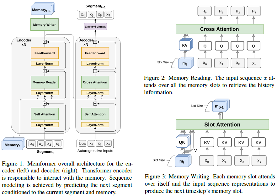
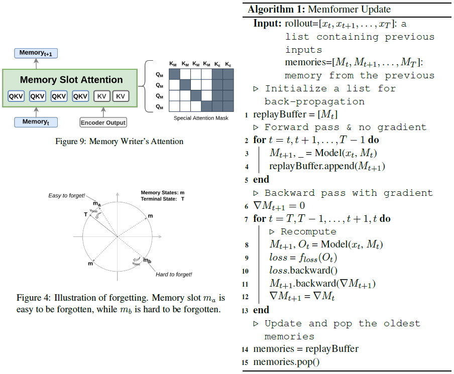
The memory writing involves a slot attention module to update memory information and a forgetting method to clean up unimportant memory information. Contrary to memory reading, memory writing only happens at the last layer of the encoder. This helps to store the high-level contextual representations into the memory. In practice, some classification tokens are appended to the input sequence to better extract the sequence representations. As shown in Figure 3 above, each slot is separately projected into queries and keys: \(Q_{m^i},K_{m^i}=m^iW_Q,m^iW_K\). The segment token representations are projected into keys and values: \(K_x,V_x=xW_K,xW_V\). In slot attention, each memory slot can only attend to itself and the token representations, but not directly attend to other slots: \(A_{m^i}^{\prime}=\mathrm{MHAttn}(Q_{m^i},[K_{m^i};K_x])\). This is implemented using a special type of sparse attention pattern (Figure 9 below). The final attention scores are computed by dividing the raw attention with a temperature \(\tau\) (\(\tau <1\)), to sharpen the attention distribution and focus on fewer slots or token outputs: \(A_{m^i}=\frac{\exp(A_{m^i}^{\prime}/\tau)}{\sum_j\exp(A_{m^j}^{\prime}/\tau)}\). The next timestep’s memory is \({m_{t+1}^i}^{\prime}=\mathrm{Softmax}(A_{x,M})[m_t^i;V_x]\). The attention mechanism helps each memory slot to choose to whether preserve its old information or update with the new information.
A forgetting mechanism called Biased Memory Normalization (BMN) is introduced for slot memory representations. The memory slots are normalized for every step to prevent memory weights from growing infinitely and maintain gradient stability over long timesteps. A learnable bias vector \(v_{bias}\) is added to each memory slot to help forget previous information: \(m_{t+1}^i\leftarrow m_{t+1}^i+v_{bias}^i\), \(m_{t+1}^i\leftarrow\frac{m_{t+1}^i}{\Vert m_{t+1}^i\Vert}\). The initial state of a memory slot is set as normalized \(v_{bias}\): \(m_0^i\leftarrow\frac{v_{bias}^i}{\Vert v_{bias}^i\Vert}\). Because of the normalization, all memory slots will be projected onto a sphere distribution. When adding \(v_{bias}\) to the memory slot, it would cause the memory to move along the sphere and forget part of its information. If a memory slot is not updated for many timesteps, it will eventually reach the terminal state \(T\) that is also the initial state and is learnable. The speed of forgetting is controlled by the magnitude of \(v_{bias}\) and the cosine distance between \(m_{t+1}^{\prime}\) and \(v_{bias}\). As the examples in Figure 4 below, \(m_b\) is nearly opposite to the terminal state, and thus would be hard to forget its information, while \(m_a\) is closer to the terminal state and thus easier to forget.
This learnable memory design requires back-propagation through time (BPTT) over a long range of timesteps so that the memory writer network can be trained to retain long-term information. The problem with traditional BPTT is that it unrolls the entire computational graph during the forward pass and stores all the intermediate activations. This process would lead to impractically huge memory consumption for Memformer. To eliminate this problem, Memory Replay Back-Propagation (MRBP) method is introduced to replay the memory at each timestep to accomplish gradient back-propagation over long unrolls. MRBP is designed specifically for recurrent neural networks. The algorithm takes an input with a rollout \(x_t\), \(x_{t+1}\),…, \(x_T\) and the previous memory \(M_t, M_{t+1},...,M_T\), if already computed. MRBP only traverses the critical path in the computational graph during the forward pass to obtain each timestep’s memory and store those memories in the replay buffer. During the backward pass, MRBP backtracks the memories in the replay buffer from time \(T\) to \(t\) and recomputes the partial computational graph for the local timestep. It continues the computation of the remaining graph with the output \(O_t\) to get the loss for back-propagation. There are two directions of gradients for the model. One direction of gradients comes from the local back-propagation of loss, while the other part comes from the back-propagation of the next memory’s Jacobin \(\bigtriangledown M_{t+1}\). The full algorithm is shown below.
Transformer-XL and Compressive Transformer use limited-length FIFO queue to store past hidden states as memories. If a sequence is longer than the maximum temporal range, the models will lose information when the stored memories are discarded. Transformer-XL has a memory cost of \(O(K\times L)\), where \(K\) is the memory size, and \(L\) is the number of layers. Compressive Transformer extends the memory cost to \(O((K+K_{cm})\times L)\), by compressing the memories in Transformer-XL into the new compressed memories with a size of \(K_{cm}\) using a compression ratio \(c\). Memformer only stores \(K\) vectors to be shared by all layers, thus with memory cost of \(O(K)\).
WikiText-103 dataset, containing 28K articles with an average of 3.6K tokens per article, is used for all language modeling experiments in this paper. Byte pair encoding (BPE) is applied to avoid unknown tokens. Different from the attention length of 1,600 tokens in the original Transformer-XL and Compressive Transformer, this study uses much smaller input size of 128 and memory size of 512, compressed memory size of 512, and compression ratio of 4. Baseline models include Transformer-XL base (\(L=16\)) and Compressive Transformer (\(L=16\)). Memformer Encoder-Decoder has \(L_{encoder}=4\) and \(L_{decoder}=16\). For fair comparison, all models have \(d_{hidden}=512\), \(d_{ff}=2048\), \(N_{heads}=8\), \(d_{head}=64\). The number of inference FLOPs and perplexity median from three trials are used as evaluation metrics. As Transformer-XL’s memory size increased from 32 to 1600, the perplexity dropped as expected, but the number of FLOPs grew quickly because the attention length was also increased. Compressive Transformer achieves slightly better performance with extra FLOPS compared to Transformer-XL with memory size 1024. Memformer with encoders \(L=4\), decoder \(L=16\), and memory size 1,024 significantly outperforms Transformer-XL with memory size 1024, using much less computation cost. Ablation studies by reducing decoder layers (\(L_{encoder}=4\) and \(L_{decoder}=12\)), reducing memory size to 512, or completely removing memory module significantly reduce perplexity performance of Memformer.
Analyses of normalized attention values in the attention outputs from the memory writer reveal that there are three types of memory slots: (1) majority (60%~80%) of the memory slots during the middle of processing a document focus attention on themselves, meaning not updating for the current timestep; (2) the second type of slots have some partial attention over itself and the rest of attention over other tokens, as if they are aggregating information from other tokens at the current timestep; (3) the third type of slots completely attend to the input tokens, such as named entities and verbs. The third type of slots have larger magnitudes in their forgetting vectors’ bias, suggesting that these memory slots change repidly.
Infinite Memory Transformer
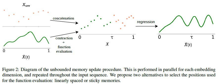
Martins et al. (2021)[22] introduced \(\infty\)-former that extends Transformer with an unbounded long-term memory (LTM) at each layer, using a continuous-space attention framework[23] that trades off the number of tokens stored into memory (basis functions) with the granularity of their representations. In this framework, the input sequence is represented as a continuous signal, expressed as a linear combination of radial basis functions (RBFs). The input context with length \(L\) can be represented using \(N\) number of basis functions, where \(N<L\); thus, reducing attention complexity. The \(N\) can be fixed, making it possible to represent unbounded context in memory without increasing its attention complexity, \(O(L^2+L\times N)\), at the cost of losing resolution. The concept of “sticky memories” is introduced to mitigate the problem of losing resolution for old memories, which attributes larger spaces in the LTM’s new signal to the relevant regions of the previous memory’s signal.
In Transformer, self-attention linearly projects the input sequence \(X=[x_1,...,x_L]\in\mathrm{\mathbb{R}}^{L\times e}\), where \(e\) is the embedding size of the attention layer, to queries \(Q=XW^Q\), keys \(K=XW^K\), and Values \(V=XW^V\), where \(W^Q,W^K,W^V\in\mathrm{\mathbb{R}}^{e\times e}\) are learnable projection matrices. In multi-head self-attention, \(Q\), \(K\), and \(V\) are split into \(H\) number of heads \(Q_h\), \(K_h\), \(V_h\in\mathrm{\mathbb{R}}^{L\times d}\) for \(h\in\{1,...,H\}\) where \(d=e/H\) is the dimension of each head. Then, the context representation \(Z_h\in\mathrm{\mathbb{R}}^{L\times d}\) from an attention head \(h\) is \(Z_h=\mathrm{softmax}(\frac{Q_hK_h^{\top}}{\sqrt{d}})V_h\) where the softmax is performed row-wise. The \(Z_h\) are concatenated to obtain the final context representation \(Z\in\mathrm{\mathbb{R}}^{L\times e}\): \(Z=[Z_1,...,Z_H]W^R\), where \(W^R\in\mathrm{\mathbb{R}}^{e\times e}\) is another projection matrix that aggregates all head’s representations.
In continuous attention, the discrete text sequence representation \(X\in\mathrm{\mathbb{R}}^{L\times e}\) is first transformed into a continuous signal by expressing it as a linear combination of basis functions. Each \(x_i\) for \(i\in\{1,...,L\}\) is first associated with a position \(t_i\in [0,1]\), e.g., by setting \(t_i=i/L\). Then, a continuous-space representation, i.e., continuous signal, \(\bar{X}(t)\in\mathrm{\mathbb{R}}^e\) for any \(t\in[0,1]\) is obtained by \(\bar{X}(t)=B^{\top}\psi(t)\), where \(B\in\mathrm{\mathbb{R}}^{N\times e}\) is a coefficient matrix and \(\psi(t)\in\mathrm{\mathbb{R}}^N\) are \(N\) 1D RBFs located in \([0,1]\). The \(B\) is obtained with a multivariate ridge regression criterion so that \(\bar{X}(t_i)\approx x_i\) for each \(i\in[L]\), which leads to the closed form: \(B^{\top}=X^{\top}F^{\top}(FF^{\top}+\lambda I)^{-1}=X^{\top}G\), where \(F=[\psi(t_1),...,\psi(t_L)]\in\mathrm{\mathbb{R}}^{N\times L}\) packs the basis vectors for the \(L\) locations. \(F\) and \(G\in\mathrm{\mathbb{R}}^{L\times N}\) can be computed offline. To do continuous attention over \(\bar{X}(t)\), a probability density \(p\), such as Gaussian \(\mathcal{N}(t;\mu,\sigma^2)\), is used, where \(\mu\) and \(\sigma^2\) are computed by a neural component. Finally, the context vector \(c\) can be computed as \(c=\mathrm{\mathbb{E}}_p[\bar{X}(t)]\).
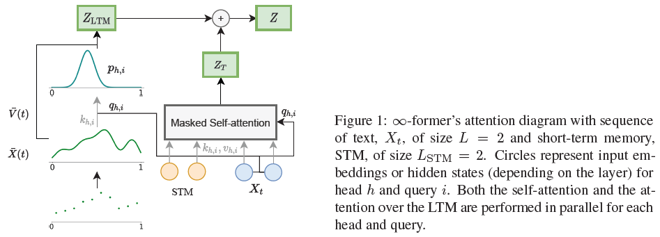
In \(\infty\)-former, as illustrated in the Figure below, it is first assumed that the LTM contains an explicit input discrete sequence \(X\) that consists of the past text sequence’s input embeddings or hidden states, depending on the layer. Each layer has a different LTM; the gradient with respect to the word embeddings or hidden states are stopped before storing them in the LTM. The \(X\) is transformed into a continuous approximation \(\bar{X}(t)\) by \(\bar{X}(t)=B^{\top}\psi(t)\), where \(\psi(t)\in\mathrm{\mathbb{R}}^N\) are basis functions and coefficients \(B\in\mathrm{\mathbb{R}}^{N\times e}\) are computed as \(B^{\top}=X^{\top}G\). Then, the LTM keys \(K\in\mathrm{\mathbb{R}}^{N\times e}\) and values \(V\in\mathrm{\mathbb{R}}^{N\times e}\) are computed as \(K=BW^K, V=BW^V\), where \(W^K,W^V\in\mathrm{\mathbb{R}}^{e\times e}\) are learnable projection matrices that are not shared between layers. For each query \(q_{h,i}\) for \(i\in\{1,...,L\}\), a parameterized network takes as input the attention scores to compute \(\mu_{h,i}\in]0,1[\) and \(\sigma_{h,i}^2\in\mathrm{\mathbb{R}}_{>0}\): \(\mu_{h,i}=\mathrm{sigmoid}(\mathrm{affine}(\frac{K_h\ q_{h,i}}{\sqrt{d}}))\), \(\sigma_{h,i}^2=\mathrm{softplus}(\mathrm{affine}(\frac{K_h\ q_{h,i}}{\sqrt{d}}))\). Then, using the continuous softmax transformation[23], the probability density \(p_{h,i}\) as \(\mathcal{N}(t;\mu_{h,i},\sigma_{h,i}^2)\). Finally, given the value function \(\bar{V}_h(t)=V_h^{\top}\psi(t)\), the head-specific representation vectors are computed as: \(z_{h,i}=\mathrm{\mathbb{E}}_{p_{h,i}}[\bar{V}_h(t)]=V_h^{\top}\mathrm{\mathbb{E}}_{p_{h,i}}[\psi(t)]\), which forms the rows of the matrix \(Z_{\mathrm{LTM},h}\in\mathrm{\mathbb{R}}^{L\times d}\) that goes through an affine transformation \(Z_{\mathrm{LTM}}=[Z_{\mathrm{LTM},1},...,Z_{\mathrm{LTM},H}]W^O\). The long-term representation, \(Z_{\mathrm{LTM}}\), is then summed to the transformer context vector, \(Z_{\mathrm{T}}\), to obtain the final context representation \(Z\in\mathrm{\mathbb{R}}^{L\times e}\): \(Z=Z_{\mathrm{T}}+Z_{\mathrm{LTM}}\), which will be the input to the transformer’s feedforward layer.
The key matrix size \(K_{\mathrm{LTM},h}\in\mathrm{\mathbb{R}}^{N\times d}\) depends only on the number of basis functions, but not on the length of the context being attended to. Thus, the \(\infty\)-former’s attention complexity is also independent of the context’s length. Therefore, the \(\infty\)-former can attend to unbounded contexts without increasing the amount of computation.
To build an unbounded representation, \(M\) locations in \([0,1]\) are sampled and \(\bar{X}(t)\) are evaluated at those locations that can be linearly spaced, or sampled according to the region importance. Then, the corresponding vectors are concatenated with the new vectors coming from the short-term memory that is the same as Transformer-XL. For that, a contraction by a factor of \(\tau\in[0,1]\) is done to make room for the new vectors: \(X^{contracted}(t)=X(t/\tau)=B^{\top}\psi(t/\tau)\). Then, \(\bar{X}(t)\) are evaluated at the \(M\) locations \(0\leq t_1,t_2,...,t_M\leq\tau\) as: \(x_m=B^{\top}\psi(t_m/\tau)\), for \(m\in[M]\). The \(x_m\) vectors are used as rows of the past matrix \(X_{past}=[x_1,x_2,...,x_M]^{\top}\in\mathrm{\mathbb{R}}^{M\times e}\) that is then concatenated with the new vectors \(X_new\) to obtain \(X=[X_{past}^{\top},X_{new}^{\top}]^{\top}\in\mathrm{\mathbb{R}}^{(M+L)\times e}\). A multivariate ridge regression is performed to compute the new coefficient matrix \(B\in\mathrm{\mathbb{R}}^{N\times e}\), via \(B^{\top}=X^{\top}G\), in which the vectors in \(X_{past}\) are associated with positions in \([0,\tau]\) and the vectors in \(X_{new}\) are associated with positions in \([\tau,1]\), as illustrated in the Figure below. The vectors are considered to be linearly spaced.
The linearly spaced sampling approach above may not perform well in cases where some regions are more relevant than others. A “sticky memories” approach is introduced to deal with this issue, which samples the \(M\) locations according to the signal’s relevance at each region. To find the relevance of a region, a histogram is constructed based on the attention given to each interval of the signal on the previous step. For that, the signal is first divided into \(D\) linearly spaced bins \(\{d_1,...,d_D\}\). Then, the probability given to each bin, \(p(d_j)\) for \(j\in\{1,...,D\}\), is computed as \(p(d_j)\propto\sum\limits_{h=1}^H\sum\limits_{i=1}^L\int_{d_j}\mathcal{N}(t;\mu_{h,i},\sigma_{h,i}^2)dt\), where \(H\) is the number of attention heads and \(L\) is the sequence length. The integral can be evaluated efficiently using the erf function: \(\int_a^b\mathcal{N}(t;\mu,\sigma^2)=\frac{1}{2}(\mathrm{erf}(\frac{b}{\sqrt{2}})-\mathrm{erf}(\frac{a}{\sqrt{2}}))\). Then, the \(M\) locations are sampled according to the \(p(d_j)\).
A simple convolutional layer (with stride = 1 and width = 3) is used as gate to smooth the LTM’s input discrete sequence: \(\tilde{X}=\mathrm{sigmoid}(\mathrm{CNN}(X))\odot X\), before applying multivariate ridge regression to convert \(X\) into \(\bar{X}\). Given a corpus of \(T\) tokens, the language model is trained by minimizing its negative log likelihood loss: \(\mathcal{L}_{\mathrm{NLL}}=-\sum\limits_{t=0}^{T-1}\log p(x_{t+1}\vert x_t,...,x_{t-L})\). To avoid having uniform distributions over the LTM, the continuous attention given to the LTM is regularized by minimizing the Kullback-Leibler (KL) divergence, \(D_{KL}\), between the attention probability density, \(\mathcal{N}(\mu_h,\sigma_h)\), and a Gaussian prior, \(\mathcal{N}(\mu_0,\sigma_0)\). As different heads should attend to different regions, \(\mu_0=\mu_h\) can be set to regularize only the attention variance: \(\mathcal{L}_{\mathrm{KL}}=\sum\limits_{t=0}^{T-1}\sum\limits_{h=1}^H D_{\mathrm{KL}}(\mathcal{N}(\mu_h,\sigma_h)\Vert\mathcal{N}(\mu_h,\sigma_0))=\sum\limits_{t=0}^{T-1}\sum\limits_{h=1}^H\frac{1}{2}(\frac{\sigma_h^2}{\sigma_0^2}-\log(\frac{\sigma_h}{\sigma_0})-1)\). Thus, the final loss to minimize is \(\mathcal{L}=\mathcal{L}_{\mathrm{NLL}}+\lambda_{\mathrm{KL}}\mathcal{L}_{\mathrm{KL}}\), where \(\lambda_{\mathrm{KL}}\) is a hyperparameter that controls the amount of KL regularization.
The Transformer-XL and the Compressive Transformer are used as baselines in this paper, both of which used relative positional encodings. In contrast, there is no need for positional encodings in the memory of \(\infty\)-former because the memory vectors represent basis coefficients in a predefined continuous space.
The first experiment is to sort tokens by their frequencies in a long sequence, e.g., \(1\ 2\ 1\ 3\ 1\ 0\ 3\ 1\ 3\ 2\ \mathrm{<SEP>}\ 1\ 3\ 2\ 0\). The input consists of a sequence of tokens sampled according to a token probability distribution, not known to the system. The objective is to generate the tokens in the decreasing order of their frequencies in the sequence. The token probability distribution is designed to change over time: \(p=\alpha p_0+(1+\alpha)p_1\), where the mixture coefficient \(\alpha\in[0,1]\) is progressively increased from 0 to 1 as the sequence is generated. The vocabulary has 20 tokens and sequence lengths of 4,000, 8,000, and 16,000 are experimented. Transformer in this experiment has 3 layers, 6 attention heads, 1,024 input length, and 2,048 memory size. For the Compressive Transformer, both memories have size of 1,024. For the \(\infty\)-former, a STM of size 1,024 and a LTM with 1,024 Gaussian RBFs \(\mathcal{N}(t;\tilde{\mu},\tilde{\sigma}^2)\) with \(\tilde{\mu}\) linearly spaced in [0,1] and \(\tilde{\sigma}\in\{0.01,0.05\}\), \(\tau=0.75\), \(\lambda_{\mathrm{KL}}=1\times 10^{-5}\), and \(\sigma_0=0.05\). For shorter sequence length (4,000), the Transformer-XL slightly outperforms the Compressive Transformer and the \(\infty\)-former, because the Transformer-XL is able to keep almost the entire sequence in memory. As the sequence length increases (8,000, and 16,000), the sorting task accuracy decreases in all three models. However, this decrease is not so significant for \(\infty\)-former and \(\infty\)-former significantly outperforms the Compressive Transformer that in turn substantially outperforms Transformer-XL, indicating that it is better at modeling long sequences.
The second experiment is language modeling on the Wikitext-103 dataset. The Transformer-XL contains 16 layers, 10 attention heads, embedding size 410, feed-forward hidden size 2,100, and memory size 150. The Compressive Transformer has a compression rate of 4 and memory size of 150 for both memories. The \(\infty\)-former has STM size of 150, LTM with 150 Gaussian RBFs, \(\tau=0.5\), \(\sigma_0=0.1\), and a memory threshold of 900 tokens. Extending the model with a long-term memory leads to a better perplexity for both Compressive Transformer and \(\infty\)-former, with \(\infty\)-former slightly better than Compressive Transformer. Using sticky memories leads to slightly better perplexity. Histograms of attention given to the LTM by \(\infty\)-former for different layers show that in the first and middle layers, the \(\infty\)-former tends to focus more on the older memories, while in the last layer, the attention pattern is more uniform. Plots of memory space vs word index in the last layer’s long-term memory (after 5 updates) without or with the sticky memories show that using sticky memories does in fact attribute large spaces to old memories, creating memories that stick over time.
The third experiment fine-tunes a pre-trained language model, GPT-2 small, on Wikitext-103 or a subset of PG-19 containing the first 2,000 books of the training set. The GPT-2 small contains 12 layers, 12 attention heads, input sequence length 512, LTM with 512 Gaussian RBFs, and a memory threshold of 2,048 tokens. The results show that by simply adding the long-term memory to GPT-2 and fine-tuning, the perplexity is improved on both Wikitext-103 and PG19. This shows the versatility of the \(\infty\)-former: it can be trained from scratch or used to improve a pre-trained model.
MemSizer
Zhang and Cai (2022)[18] introduced MemSizer that replaces the self-attention layer of Transformer with a novel key-value memory layer, which leads to linear time complexity in sequence length and running autoregressive sequence generation with constant memory complexity. Although MemSizer significantly reduces time and space complexities, it actually underperforms vanilla Transformer on language modeling task.
A key-value memory network projects a set of input source vectors \(\mathrm{X}^s=\{\mathrm{x}_i^s\}_{i=1}^M\) into memory key vectors \(\mathrm{K}\in\mathrm{\mathbb{R}}^{M\times h}\) and value vectors \(\mathrm{V}\in\mathrm{\mathbb{R}}^{N\times h}\). A target vector \(\mathrm{x}^t\) is also projected to a query vector \(\mathrm{q}\in\mathrm{\mathbb{R}}^{h}\) in the same embedding space as key vectors. Then, a probability vector \(\alpha\) is computed based on inner product similarity: \(\alpha=f(\mathrm{qK}^{\top})\), where \(f\) denotes an activation function, typically softmax function. The output vector \(\mathrm{x}^{out}\) of a layer is simply summarizing over the value vectors according to their probabilities: \(\mathrm{x}^{out}=\alpha\mathrm{V}\).
The multi-head self-attention layer in a Transformer maps input vectors \(\mathrm{X}^s\in\mathrm{\mathbb{R}}^{M\times d}\) and target vectors \(\mathrm{X}^t\in\mathrm{\mathbb{R}}^{N\times d}\), where \(d\) is the model dimension, to \(\mathrm{Q}=\mathrm{X}^t\mathrm{W}_q+\mathrm{b}_q\), \(\mathrm{K}=\mathrm{X}^s\mathrm{W}_k+\mathrm{b}_k\), and \(\mathrm{V}=\mathrm{X}^s\mathrm{W}_v+\mathrm{b}_v\), where \(\mathrm{W}_*\in\mathrm{\mathbb{R}}^{d\times h}\), \(\mathrm{b}_*\in\mathrm{\mathbb{R}}^{h}\), and \(h\) is the dimension of the query, key, value vectors. The number of attention heads \(r=\frac{d}{h}\). The attention weight \(\alpha\) is the normalized similarities between query vectors and key vectors: \(\alpha=\mathrm{softmax}({\frac{\mathrm{Q}\mathrm{K}^{\top}}{\sqrt{h}}})\). The output of each head \(\mathrm{X}_{(i)}^{out}\) is a weighted average of the value vectors \(\mathrm{X}_{(i)}^{out}=\alpha\mathrm{V}\). The output vectors of the \(r\) heads are concatenated to get the final vector: \(\mathrm{X}^{out}=[\mathrm{X}_{(1)}^{out},...,\mathrm{X}_{(r)}^{out}]W_o+b_o\), where \(W_o\in\mathrm{\mathbb{R}}^{d\times d}\) and \(b_o\in\mathrm{\mathbb{R}}^{d}\) are the output projection weights. The self-attention in the Transformer can be perceived as an instance of the key-value memory network described above, where the memory keys \(\mathrm{K}\) and values \(\mathrm{V}\) are projections of the source \(\mathrm{X}^s\).
MemSizer replaces the self-attention layer in Transformer with a different specifications of query, key, and value of a key-value memory layer: \(\mathrm{Q}=\mathrm{X}^t\), \(\mathrm{K}=\Phi\), \(\mathrm{V}=\mathrm{LN}(\mathrm{W}_l(\mathrm{X}^s)^{\top})\mathrm{LN}(\mathrm{X}^s\mathrm{W}_r)\). The key matrix \(\Phi\in\mathrm{\mathbb{R}}^{k\times d}\) is a learnable matrix shared across different input instances, where \(k\) is the number of memory slots. The source information \(\mathrm{X}^s\) is encoded into the value matrix \(\mathrm{V}\in\mathrm{\mathbb{R}}^{k\times d}\) via two adaptor weights \(\mathrm{W}_l\in\mathrm{\mathbb{R}}^{k\times d}\) and \(\mathrm{W}_r\in\mathrm{\mathbb{R}}^{d\times d}\) that project source information into global representation \(\mathrm{\mathbb{R}}^{k\times d}\) regardless of the input length \(M\) and \(N\). The \(\mathrm{LN}(\cdot)\) denotes the layer normalization, which makes the training robust. To control the magnitude of \(\mathrm{V}\) across variable-length input sequences, the \(\mathrm{V}\) is multiplied by a scaling factor of \(1/\sqrt{M}\). The memory layer is made multi-head by sharing \(\mathrm{V}\) across \(r\) different heads but using a distinct \(\mathrm{K}\) for each head, unlike vanilla Transformer’s \(d=hr\). The outputs from multi-head are then aggregated through mean-pooling: \(\mathrm{X}^{out}=\frac{1}{r}\sum\limits_{i=1}^r\mathrm{X}_{(i)}^{out}\), where \(\mathrm{X}_{(i)}^{out}\) is the output from \(i\)-th head. The final output \(\mathrm{X}^{out}\) has dimension \(d\) and there is no need for output projection layer.
To perform autoregressive generation, MemSizer uses a recurrent procedure. At each generation step \(i\), define \(\mathrm{V}_{i}\) as the recurrent states: \(\mathrm{V}_{i}=\sum\limits_{j=1}^i\mathrm{LN}(\mathrm{W}_l(\mathrm{x}_j^s)^{\top})\mathrm{LN}(\mathrm{x}_j^s\mathrm{W}_r)\), where \(\mathrm{x}_j^s\) is the j-th row of \(\mathrm{X}^s\) and \(\mathrm{V}_{i}\) can be perceived as a rolling-sum matrix: \(\mathrm{V}_{i}=\mathrm{V}_{i-1}+\mathrm{LN}(\mathrm{W}_l(\mathrm{x}_j^s)^{\top})\mathrm{LN}(\mathrm{x}_j^s\mathrm{W}_r)\). Thus, the output \(\mathrm{X}_{i}^{out}\) can be computed in an incremental manner from cached recurrent matrix \(\mathrm{V}_{i-1}\). This avoids quadratic computation overhead with respect to input sequence length.
The generation time complexity of MemSizer is \(O(Mdk+Md^2+Ndk)\), linear with respect to input length \(M\) and \(N\), as opposed to \(O(MNd+Md^2+Nd^2)\) of the self-attention. MemSizer memory only needs to store the value matrix \(\mathrm{V}\); thus, the generation memory space complexity is \(O(dk)\), constant with respect to input length. The \(k\) can be arbitrarily configured to balance between performance and efficiency. In MemSizer, each memory slot value \(\mathrm{v}_{j\in\{1,...,k\}}\) summarizes a global position-agnostic feature of the source context \(X^s\).
The WikiText-103 dataset is used to evaluate language modeling, with hyperparameters: 32 layers, 8 heads, 128 head dimensions, 1024 model dimensions, 4096 fully connected dimensions, 0.2 dropout, and memory size \(k\)=32. The word embedding and softmax matrices are tied. Validation and test perplexity is measured by predicting the last 256 words out of the input of 512 consecutive words to avoid evaluating tokens in the beginning with limited context.
The WMT16 En-De, WMT14En-Fr, and WMT17 Zh-En datasets are used to evaluate machine translation (MT), with hyperparameters (for both encoder and decoder): 6 layers, 16 attention heads, 1024 model attentions, 4096 hidden dimensions, and 0.3 dropout. Beam search is used for decoding with beam size 5 and length penalty 1.0. Tokenized BLEU is used for evaluation. MemSizer is applied to both cross and causal attention in MT. Memory size \(k\) is 32 and 4 for cross and causal attention, respectively.
Three previous recurrent Transformer models with linear time and constant space complexity with respect to sequence length are used as baseline models: ELU, RFA, and T2R. These models approximate the softmax attention kernel between \(\mathrm{q}\) and \(\mathrm{k}\) by projecting them via feature map function \(\phi(\cdot)\). ELU uses exponential linear unit: \(\phi(x)=\mathrm{elu}(x)+1\)[19]. RFA uses a random feature map with softmax temperature reparameterization[20]. T2R uses trainable feature mapping which allows smaller feature size thus further improving the efficiency[21]. Approximating self-attention softmax kernel typically needs additional steps to obtain intermediate feature mapping results. MemSizer employs a key-value memory module to avoid these intermediate steps and the output projection step in self-attention.
Language modeling results show that MemSizer outperforms ELU and RFA, and achieves comparable performance to T2R, but substantially underperforms vanilla Transformer. MemSizer also shows significantly faster generation speed and significantly smaller memory usage and model size than the three baseline models and vanilla Transformer. Machine translations results show that MemSizer, with ~17% smaller model size, outperforms RFA and T2R while being comparable to ELU in En-De and outperforms all baseline methods in En-Fr and Zh-En. Thus, MemSizer provides an improved tradeoff between accuracy of the vanilla transformer and efficiency of linear variants in language modeling and machine translation tasks.
MemSizer can generate a nearly constant number of tokens per second regardless of the sequence length, but vanilla transformer model becomes much slower at longer sequence. At 512 input sequence length for MT in En-De, MemSizer speed is about 20,000 tokens/s and Transformer speed is about 5,000 tokens/s. MemSizer also substantially outpaces the three linear recurrent baseline models, with the maximum speedup at length 64. The decoder memory consumption for MT in En-De is almost a constant over varying sequence lengths and is lower than other baselines consistently.
Increasing the number of memory slots \(k\) (ranging from 8 to 128), improves the performance on the language modeling task, without considerable impact on time and memory cost. However, during training time, processing time per tokens are roughly linear to k, presumably because more intermediate states need to be stored for back-propagation. The number of attention heads slightly affects the test perplexity on the language modeling task, resulting in slightly better performance with more attention heads, without significant difference in training and inference overhead, as the multi-head computation is lightweight in MemSizer.
The importance of trainable memory keys \(\mathrm{K}\) is studied by initializing \(\mathrm{K}\) for each layer and each head with standard Xavier initialization and freezing them during the training process. In both language modeling and machine translation tasks, the performance dropped with a relatively small margin. As \(k\ll d\), the keys in \(\mathrm{K}\) almost orthogonal with Xavier initialization, thus less likely to “collide” with each other. Therefore, updating \(\mathrm{K}\) becomes less essential comparing to other parts of model.
Special Input Tokens as Memory
Using tokens as memory is a simple way to extract global context information, but its benefit is relatively small and inconsistent, probably because the number of tokens is limited.
MemTransformer
Burtsev et al. (2020)[15] introduced Memory Transformer (MemTransformer) that extends Transformers by adding \([\mathrm{mem}]\) tokens at the beginning of the input sequence for storing non-local representations. Two additional variants of MemTransformer are also examined: MemCtrl Transformer that uses a dedicated subnetwork for processing \([\mathrm{mem}]\) tokens and MemBottleneck Transformer that processes \([\mathrm{mem}]\) tokens and input sequence of each layer in two stages, as illustrated in the Figure below.
![]()
In a single Transformer layer, multi-head attention \(MH(Q,K,V)\) output and skip-connected input \(X\) are summed up and layer-normalized (LN) to obtain aggregated representations \(A=LN(X+MH(X,X,X))\) that is then passed through fully-connected feed-forward (FF) sub-layer to obtain hidden state output of the layer \(H=LN(A+FF(A))\). In single MemTransformer layer, \(m\) special \([\mathrm{mem}]\) tokens \(X^{mem}\in\mathrm{\mathbb{R}}^{m\times d}\) are prepended to the standard input \(X^{seq}\in\mathrm{\mathbb{R}}^{n\times d}\) and the concatenated input \(X^{mem+seq}=[X^{mem};X^{seq}]\in\mathrm{\mathbb{R}}^{(m+n)\times d}\) is processed in the same standard way. In single MemCtrl Transformer layer, memory token representations and sequence token representations are processed by different subnetworks: \(A^{mem}=LN(X^{mem}+MH^{mem}(X^{mem},X^{mem+seq},X^{mem+seq}))\), \(H^{mem}=LN(A^{mem}+FF^{mem}(A^{mem}))\) for memory token representations, and \(A^{seq}=LN(X^{seq}+MH^{seq}(X^{seq},X^{mem+seq},X^{mem+seq}))\), \(H^{seq}=LN(A^{seq}+FF^{seq}(A^{seq}))\) for sequence token representations. In single MemBottleneck Transformer layer, memory token representations and sequence token representations are processed not only by different subnetworks, but also in sequential fashion: the memory token subnetwork is identical to those in MemCtrl Transformer, but the sequence token subnetwork uses the output hidden states of memory tokens as input for multi-head attention, \(A^{seq}=LN(X^{seq}+MH^{seq}(X^{seq},H^{mem},H^{mem}))\) and \(H^{seq}=LN(A^{seq}+FF^{seq}(A^{seq}))\). For all encoder-decoder variants of the memory transformers the decoder part is the same as in the baseline. Output of the last encoder layer [$$H^{mem};H^{seq}] is passed to the decoder layers.
Machine translation (MT), language modeling (LM), and language understanding (LU) tasks are used for evaluation. For ML task, a vanilla encoder-decoder Transformer is used as a reference model. For LM task, Transformer-XL is augmented with 20 \([\mathrm{mem}]\) tokens. For LU tasks, pre-trained BERT is augmented.
BLEU 4 scores of WMT-14 DE-EN translation task show that MemTransformer outperforms reference model and the performance improvement increases as the number of prepended \([\mathrm{mem}]\) tokens increases on 6-6-layer model, but not on 4-4-layer model. MemCtrl Transformer underperforms reference model, but outperforms it when all 6 encoder layers share parameters. MemBottleneck substantially underperforms reference model. Changing the number of prepended \([\mathrm{mem}]\) tokens at inference time to be different from the number at training time show that both decreasing and increasing \([\mathrm{mem}]\) tokens at inference time reduce performance and the extent of reduction is more prominent when the number at training time is larger. When further training is performed along with increasing \([\mathrm{mem}]\) tokens at inference time, the performance improves.
In language modeling task trained on WikiText-103, MemTransformer with 20 \([\mathrm{mem}]\) tokens modestly outperforms Transformer-XL on both word-level perplexity and character-level bits-per-character. In language understanding task on GLUE datasets, adding \([\mathrm{mem}]\) tokens to pre-trained BERT-base model modestly improves its performance on 6 of the 9 tasks.
Qualitative analysis of attention map, as illustrated in the Figure below, produced by the transformer heads trained for machine translation task reveal some attention patterns that can be interpreted as memory read/write as well as some in-memory processing operations such as copying and summation.
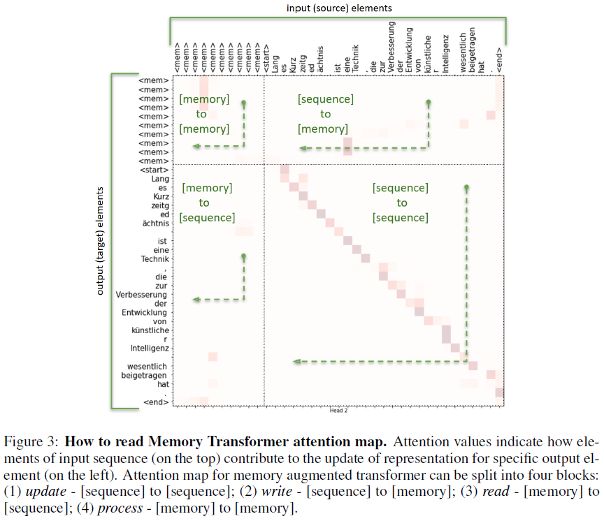
Memory Replay for Lifelong Language Learning
In natural cognitive systems, such as human brain, learning new knowledge does not cause previously learned knowledge to be erased, which makes lifelong learning (or continual learning) possible. On the contrary, artificial neural network has been shown to exhibit catastrophic forgetting (or catastrophic interference) in learning multiple tasks sequentially[32][33], where the network substantially forgets previously learned knowledge upon learning new tasks (with different data distributions) because the weights important to previous tasks are modified. Several categories of methods have been developed to avoid catastrophic forgetting (CF) in lifelong learning[34]: (1) Replay-based methods store some training data of previous tasks and replay them in training new tasks to retain old knowledge; (2) Regularization-based methods add a regularization term or an optimization constraint to the loss to prevent model parameters from changing too much; (3) Gradient-based methods ensure that weights can only be modified in the direction orthogonal to the subspace spanned by all previously learned inputs; (4) Parameter isolation-based methods dedicate different subnetworks for different tasks to prevent interference during training and use learned combinations for inference; (5) Meta-learning-based methods either directly optimize the knowledge transfer among tasks or learn data representations robust to forgetting; (6) Adapter-based methods leverages capsules and dynamic routing to identify previous tasks that are similar to the new task and exploit their shared knowledge to help the new task learning and uses task masks to protect task-specific knowledge to avoid forgetting. The replay-based methods are among the best performing methods.[36][37][49] A theoretical study[39] has concluded that perfect memory is required for an optimal continual learning algorithm. This section covers recent studies of memory-replay-based methods for lifelong language learning using Transformer-based models.
Episodic Memory Replay
Episodic memory refers to memories of past events, distinct from time-independent memories of factual knowledge[38]. It enables human mental time travel to the past and, similarly, neural network’s replay of past training examples in lifelong learning setting. Sprechmann et al. (2018)[35] introduce Memory-based Parameter Adaptation (MbPA) method that augments neural network with an episodic memory for storage of embedded training examples and, during testing, retrieves K-nearest memorized examples to a test example for local adaptation of the weights before making prediction. The MbPA substantially alleviates catastrophic forgetting in continual learning settings. de Masson d’Autume et al. (2019)[36] improve MbPA by performing sparse memory replay during training and refer to the model as MbPA++ that significantly outperforms MbPA in continual learning tasks. Wang et al. (2020)[37] improve MbPA++ by adding local adaptation in training phase using meta-learning approach and refer to the model as Meta-MbPA that outperforms MbPA++. Han et al. (2020)[46] introduce episodic memory activation and reconsolidation (EMAR) method to continual relation learning, which outperforms the then state-of-the-art continual relation learning models. Holla et al. (2020)[40] augment online meta-learning (OML) and a neuromodulatory meta-learning algorithm (ANML) with an episodic memory module for experience replay (ER) and refer to them as OML-ER and ANML-ER, respectively, which outperform MbPA++ but underperform Meta-MbPA. Qin et al. (2022)[47] expands a pre-trained language model’s width and depth for each new task and uses memory replay to “warm up” the new parameters before training the expanded model on the new task that also includes a small portion on memory replay. Domain prompts are prepended with inputs. The resulting model has high pre-training efficiency and is referred to as ELLE (Efficient LifeLong pre-training for Emerging data).
Improved MbPA
MbPA++[36] performs a sparse experience replay during training and local adaptation during inference to mitigate catastrophic forgetting in lifelong learning. At training time, newly acquired knowledge are consolidated with very sparsely replayed examples randomly selected from memory. It is shown that a 1% experience replay to learning new examples ratio is sufficient. At inference time, test input is used to retrieve relevant examples from the memory and the model parameters are updated (locally adapted) using the examples before being used to make a prediction. The lifelong learning setup in this paper assumes that the model only makes one pass over the training examples and there is no explicit identifier about the datasets (distributions) for training or testing examples. Two language learning tasks, text classification and question answering, are used for evaluation.
The model for lifelong learning needs to learn from a stream of training examples \(\{x_t,y_t\}_{t=1}^T\) from multiple datasets of the same task, coming one after another in series. The goal of the learning is to find parameters \(\mathrm{W}\) that minimize the negative log probability of training examples: \(\mathcal{L}(\mathrm{W})=-\sum\limits_{t=1}^T\log p(y_t\vert x_t;\mathrm{W})\). The model consists of three main components: (i) an example encoder, (ii) a task decoder, and (iii) an episodic memory module[35], as illustrated in the Figure below.
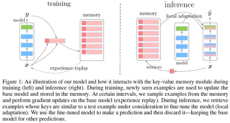
A pre-trained BERT is used as the example encoder to encode input example \(x_t\). In text classification, \(x_t\) is a document to be classified; BERT produces a vector representation for each token in \(x_t\), which includes a special beginning-of-document symbol \(\mathrm{CLS}\) as \(x_{t,0}\). In question answering, \(x_t\) is a concatenation of a context paragraph \(x_t^{\mathrm{context}}\) and a question \(x_t^{\mathrm{question}}\) separated by a special separator symbol \(\mathrm{SEP}\).
For text classification, the task decoder is a linear transformation that takes the representation of \(x_{t,0}\) from BERT as input and a softmax layer that predicts the class of \(x_{t,0}\): \(p(y_t=c\vert x_t)=\frac{\exp(\mathrm{w}_c^{\top}\mathrm{x}_{t,0})}{\sum_{y\in\mathcal{Y}}\exp(\mathrm{w}_y^{\top}\mathrm{x}_{t,0})}\). All the classes in all datasets are known in advance. For question answering, the task decoder predicts an answer span, represented as the start and end indices of the correct answer in the context, using two sets of parameters: \(\mathrm{w}_{\mathrm{start}}\) and \(\mathrm{w}_{\mathrm{end}}\). Given a context paragraph \(x_t^{\mathrm{context}}=\{x_{t,0}^{\mathrm{context}},...,x_{t,M}^{\mathrm{context}}\}\), where \(M\) is the length of the paragraph, and \(\mathrm{x}_{t,m}^{\mathrm{context}}\) as the encoded representation of the \(m\)-th token in the context, the probability of each context token being the start of the answer is computed as: \(p(\mathrm{start}=x_{t,m}^{\mathrm{context}}\vert x_t)=\frac{\exp(\mathrm{w}_{\mathrm{start}}^{\top}\mathrm{x}_{t,m}^{\mathrm{context}})}{\sum_{n=0}^M\exp(\mathrm{w}_{\mathrm{start}}^{\top}\mathrm{x}_{t,n}^{\mathrm{context}})}\). The probability of the end index of the answer is computed analogously using \(\mathrm{w}_{\mathrm{end}}\). The predicted answer is the span with the highest probability after multiplying the start and end probabilities.
The episodic memory module is a key-value memory block. Another pre-trained BERT model, different from the example encoder, is used as the key network to encode the memory key \(\mathrm{u}_t\) for the input \(x_t\). The key network is not updatable to prevent key representations from drifting as data distribution changes. For text classification, the key vector is the encoded representation of the special beginning-of-document symbol (i.e., first token of the document to be classified), \(\mathrm{u}_t=\mathrm{x}_{t,0}\). For question answering, the key vector is the encoded representation of the first token of the question part of the input, \(\mathrm{u}_t=\mathrm{x}_{t,0}^{\mathrm{question}}\). For both tasks, the memory value is the input and the label \(\langle x_t,y_t\rangle\). The memory write adopts random write strategy, where a newly seen example is written into the memory with some probability. The memory read adopts two retrieval mechanisms: random sampling and \(K\)-nearest neighbors, which are used for sparse experience replay and local adaptation, respectively. The sparse experience replay and local adaptation are used in training and inference, respectively, as illustrated in the algorithms below.
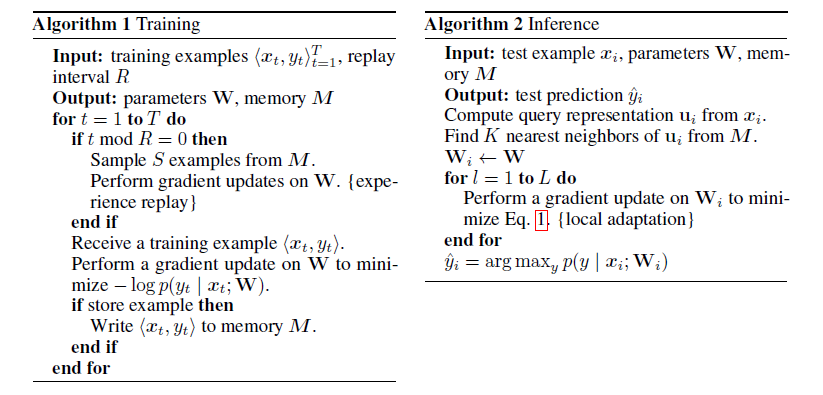
For sparse experience replay, at a certain interval during training, stored examples in the memory are randomly and uniformly sampled, and the retrieved examples are used to perform gradient updates of the example encoder-task decoder network. The experience replay procedure randomly retrieves 100 examples every 10,000 new examples. Only one gradient update is performed for the 100 retrieved examples. For local adaptation, given a test example at inference time, the key network encodes the test example into a query vector that is used to retrieve \(K\) nearest neighbors from the memory using the Euclidean distance function. The \(K\) retrieved examples \(\{x_i^k,y_i^k\}_{k=1}^K\) for the \(i\)-th test example are used to perform gradient-based local adaptation by updating the parameters of the encoder-decoder model, denoted as \(\mathrm{W}\), to obtain local parameters \(\mathrm{W}_i\) to be used for the current prediction as: \(\mathrm{W}_i=\mathrm{argmin}_{\tilde{\mathrm{W}}}\lambda\Vert\tilde{\mathrm{W}}-\mathrm{W}\Vert_2^2-\sum\limits_{k=1}^K\alpha_k\log p(y_i^k\vert x_i^k;\tilde{\mathrm{W}})\), where \(\lambda\) is a hyperparameter, \(\alpha_k\) is the weight of the \(k\)-th retrieved example and \(\sum_{k=1}^K\alpha_k=1\). It is assumed that all \(K\) retrieved examples are equally important regardless of their distance to the query vector and set \(\alpha_k=\frac{1}{K}\). The \(\mathrm{W}_i\) is only used to make a prediction for the \(i\)-the example, and the parameters are reset to \(\mathrm{W}\) afterwards. Local adaptation gradient steps are performed only \(L\) times, instead of finding the true minimum. The procedure locally adapts parameters of the encoder-decoder network to be better at predicting retrieved examples from the memory, while keeping it close to the base parameters \(\mathrm{W}\).
The datasets for text classification are from 5 diverse domains (AGNews, Yelp, Amazon, DBPedia, Yahoo), with number of classes ranging from 4 to 14 and in total of 33. A balanced version of merged dataset is created to have the same number of randomly sampled examples from each source. For question answering, 3 datasets (SQuAD 1.1, TriviaQA, QuAC) of different characteristics are used. Seven models are compared: (1) ENC-DEC, a standard encoder-decoder model without episodic memory module; (2) A-GEM[52], Average Gradient Episodic Memory model that defines constraints on the gradients that are used to update model parameters based on retrieved examples from the memory (without dataset identifier); (3) REPLAY, a model that uses stored examples for sparse experience replay without local adaptation; (4) MBPA (memory-based parameter adaptation)[35], an episodic memory model that uses stored examples for local adaptation without sparse experience replay (fixed key network variant); (5) \(\mathrm{MBPA}_{++}^{\mathrm{rand}}\), an episodic memory model with randomly retrieved examples for local adaptation (no key network); (6) MBPA++, the episodic memory model described in this paper; (7) MTL, a multitask model trained on all datasets jointly, used as a performance upper bound. The pre-trained \(\mathrm{BERT}_{\mathrm{BASE}}\) model used for example encoder and key network has 12 transformer layers, 12 self-attention heads, and 768 hidden dimensions (110M parameters in total). The number of neighbors and the number of local adaptation steps are set as \(K\) = 32 and \(L\) = 30, respectively.
For text classification, the performance is in the order: MTL > MBPA++ (this paper) > MBPA (local adaptation only) > A-GEM > \(\mathrm{MBPA}_{++}^{\mathrm{rand}}\) > REPLAY > ENC-DEC. For question answering, the performance is in the order: MTL > MBPA++ (this paper) > MBPA (local adaptation only) > \(\mathrm{MBPA}_{++}^{\mathrm{rand}}\) > REPLAY > A-GEM > ENC-DEC. Local adaptation (MBPA) and sparse experience replay (REPLAY) help mitigate catastrophic forgetting compared to ENC-DEC, but a combination of them is needed to achieve the best performance (MBPA++). The fact that MBPA++ substantially outperforms \(\mathrm{MBPA}_{++}^{\mathrm{rand}}\) indicates that retrieving relevant examples from memory is crucial to ensure that the local adaptation phase is useful. The results also suggest that MBPA++ can be improved further by choosing relevant examples for sparse experience replay. MBPA++ not only shows the ability to retain performance of previously learned dataset in lifelong learning setting, but also demonstrates the ability of positive transfer, because it substantially outperforms single-dataset models on text classification.
The effect of memory capacity is studies by comparing models that store 100%, 50%, and 10% of the training examples. For the 50% and 10% cases, examples are randomly selected for memory write with probability of 0.5 and 0.1, respectively. The results demonstrate that while the performance of the model degrades as the number of stored examples decreases, the model is still able to maintain a reasonably high performance even with only 10% memory capacity of the full model. The model performance is also improved as the number of retrieved memory examples for local adaptation is increased.
The run time cost of memory replay in training is negligible because it is performed sparsely (1%), but the memory incurs higher space complexity. The local adaptation does reduce inference speed. The number of local adaptation steps needs to be at least 15 to have optimal performance; thus, this model has a slower inference speed.
Meta-MbPA
Meta-MbPA[37] addresses three drawbacks of MbPA++: (1) To achieve optimal performance, it needs to store all training examples, which requires an unrealistically large memory module. (2) The local adaptation steps required for each test example make the inference speed extremely slow. (3) The local adaptation is prone to negative transfer that causes a lower performance on the most recent task in a sequence of tasks. The negative transfer refers to the phenomenon that a model fails to effectively reuse previously acquired knowledge to help learn new tasks. In local adaptation, the negative transfer is likely caused by overfitting the model with examples retrieved from memory and thus hurting the performance on examples from new task, which is more significant when the memory size is small. In MbPA++, the negative transfer may be attributed to a discrepancy between training and testing, where local adaptation is not applied during training, but applied before each testing example. Thus, MbPA++ always overfits to the latest task it has been trained on, and it never learns how to incorporate memory replay efficiently.
Three improvements are included in Meta-MbPA: (1) To reduce memory size, a diversity-based selection criterion is used to determine whether a training example will be added into memory. (2) Local adaptation is applied to training stage for both training examples and replayed memory examples. (3) A coarse local adaptation is used to alleviate negative transfer due to small memory size.
During training, the model makes a single pass over the training example stream consisting of \(N\) tasks in an ordered sequence, \(\mathcal{D}^{train}=\{\mathcal{D}_1^{train},...,\mathcal{D}_N^{train}\}\), where \(\mathcal{D}_t^{train}=\{(x_t^i,y_t^i)\}_{i=1}^{n_t}\) is drawn from the task-specific distribution \(P_t(\mathcal{X},\mathcal{Y})\) of the \(t\)-th task. The diversity-based selection criterion exploits the key network \(g_{\phi}\) to estimate diversity via the minimum distance of \(x_t^i\) to existing memory as: \(\log(p(x_t^i))\propto -\frac{\min\limits_{x,y\in\mathcal{M}}\Vert g_{\phi}(x_t^i)-g_{\phi}(x)\Vert_2^2}{\beta}\), where \(p(x_t^i)\) is the probability of the training example \((x_t^i,y_t^i)\in\mathcal{D}^{train}\) being selected to be added to the memory and \(\beta\) is a scaling parameter (\(\beta=10\)). The idea is to select examples that are less similar to existing memory thereby covering diverse part of data distribution.
To incorporate local adaptation into training stage, the idea of meta training is exploited by formulating local adaptation as the base task and representation learning as the meta task. The generic representation is trained such that it should perform well after the local adaptation, a.k.a. learning to adapt. Thus, for each training example \((x_t^i,y_t^i)\in\mathcal{D}^{train}\), the original task loss \(\mathcal{L}_{\mathrm{TASK}}(\theta;x_t^i,y_t^i)=\mathcal{l}(f_{\theta}(x_t^i),y_t^i)\) of MbPA++, where \(f_{\theta}\) is the predictor network, is formulated into a meta-task loss as: \(\mathcal{L}_{\mathrm{TASK}}^{\mathrm{meta}}(\theta;x_t^i,y_t^i)=\mathcal{l}(f_{\tilde{\theta}_{x_t^i}}(x_t^i),y_t^i)\) s.t. \(\tilde{\theta}_{x_t^i}=\theta -\alpha\nabla_{\theta}\mathcal{L}_{\mathrm{LA}}(\theta;\mathcal{N}_{x_t^i})\), where \(\alpha\) is the current learning rate (\(\alpha=1e^{-5}\)) and \(\mathcal{N}_{x_t^i}\) is the \(K\) nearest neighbor context of the \(i\)-th training example of the \(t\)-th task \(x_t^i\). The differentiation requires computing the gradient of gradient, which can be implemented by modern automatic differentiation frameworks (PyTorch is used in this study). The local adaptation is approximated first using gradient steps, and then the adapted network is optimized. Similarly, the original memory reply loss \(\mathcal{L}_{\mathrm{REP}}(\theta;\mathcal{S})=\frac{1}{n_{re}}\sum\limits_{x,y\in\mathcal{S}}\mathcal{l}(f_{\theta}(x),y)\) of MbPA++, where \(\mathcal{S}\) is a subset of memory and \(n_{re}\) is the number of examples in \(\mathcal{S}\) selected (randomly in MbPA++) from memory for replay, is reformulated into a meta-replay loss: \(\mathcal{L}_{\mathrm{REP}}^{\mathrm{meta}}(\theta;\mathcal{S})=\frac{1}{n_{re}}\sum\limits_{x,y\in\mathcal{S}}\mathcal{l}(f_{\tilde{\theta}_x}(x),y)\) s.t. \(\tilde{\theta}_x=\theta -\alpha\nabla_{\theta}\mathcal{L}_{\mathrm{LA}}(\theta;\mathcal{N}_x)\) with the objective to stimulate efficient local adaptation for all tasks. The same replay ratio, 1%, as in MbPA++ is used to keep the meta replay sparse.
At inference time in MbPA++, the key network \(g_{\phi}\), which is fixed during training, is used to encode example inputs as keys to obtain the \(K\) nearest neighbor context \(\mathcal{N}_{x_i}\) of the \(i\)-th testing example \(x_i\). \(L\) local adaptation gradient updates are then performed to achieve task-specific finetuning for the following objective: \(\mathcal{L}_{\mathrm{LA}}(\tilde{\theta}_i;\theta,\mathcal{N}_{x_i})=\frac{1}{K}\sum\limits_{x,y\in\mathcal{N}_{x_i}}\mathcal{l}(f_{\tilde{\theta}_i}(x),y)+\lambda_l\Vert\tilde{\theta}_i-\theta\Vert_2^2\), where \(\lambda_l\) is a hyperparameter (\(\lambda_l=0.001\)). The predictor network \(f_{\tilde{\theta}_i}\) is then used to output the final prediction for the \(i\)-th testing example. With small memory, local adaptation for each testing example is prone to negative transfer, because less related memory samples are more likely to be included in \(\mathcal{N}_{x_i}\) and the model can easily overfit. Thus, local adaptation in Meta-MbPA is done with more coarse granularity, which uses the same \(L=30\) local adaptation update steps for whole testing set (i.e., local adaptation is performed only once for the entire testing set).
The datasets used in this study are the same as those used in MbPA++. The baseline models include (1) a standard encoder-decoder without any regularization, (2) Online EWC[54] and (3) A-GEM[52] with parameter regularization, (4) REPLAY with sparse memory replay only, and (5) MbPA++ with memory replay and local adaptation. Pre-trained \(\mathrm{BERT}_{\mathrm{BASE}}\) (12 layers, 12 heads, 768 hidden dimensions, 110M parameters) is used for initializing the encoder network. A separate pre-trained \(\mathrm{BERT}_{\mathrm{BASE}}\) is used for key network and freeze it to prevent from drifting while training on a non-stationary data distribution. Faiss is used for efficient nearest neighbor search in memory. The memory size is controlled through a write rate \(r_{\mathcal{M}}=1\%\). The number of neighbors is set as \(K=32\).
Even using only 1% of total training examples as memory, Meta-MbPA still outperforms all baselines that use all training examples as memory, on both text classification and question answering tasks. Regularization-based methods (Online EWC and A-GEM) perform better than the standard Enc-Dec model, but their performance vary depending on the task ordering and thus are not robust. On the other hand, methods that involve local adaptation (MbPA++ and Meta-MbPA) perform consistently better for all orderings. In particular, Meta-MbPA improves over MbPA++ while using 100 times less memory, indicating that Meta-MbPA can utilize the memory module more effectively. Comparing to the multitask model MTL, Meta-MbPA (1% memory) still underperforms MTL (100% memory).
Four memory selection methods are compared: random selection, diversity-based method used in this study, and two uncertainty-based methods that picks the most unsure examples: “Uncertainty” utilizing model’s confidence level and “Forgettable” selecting examples according to forgetting events. The diversity-based method slightly outperforms random selection that in turn substantially outperforms the two uncertainty-based methods. Inspecting which tasks each testing example’s retrieved neighbors come from during the local adaptation phase reveals that more examples from other tasks are used as nearest neighbors when models use uncertainty-based methods. This is because the selected uncertain examples are usually less representative in the true distribution and the resulting memory does not have a good coverage of the data distribution. Consequently, less related examples from other tasks are used for the local adaptation, which causes negative transfer. Both MbPA++ and Meta-MbPA using the uncertainty-based memory selection methods without local adaptation outperform their locally adapted counterparts. But the performance gap is much smaller in Meta-MbPA, indicating that it is less susceptible to negative transfer.
This study shows that there is a trade-off between catastrophic forgetting and negative transfer, such that more adaptations are desired for earlier tasks while less is better for later tasks. The standard Enc-Dec model performs poorly on previously trained tasks, indicating the occurrence of catastrophic forgetting. On the contrary, the standard Enc-Dec and REPLAY models perform best on the last task across all four task orderings, suggesting that local adaptation, especially in MbPA++, causes negative transfer. On the other hand, the Meta-MbPA is trained to learn a more robust initialization for adaptation and uses a coarse adaptation that is less prone to negative transfer. Ablation study shows the order of importance: meta learning mechanism \(>\) local adaptation \(>\) memory selection method. The coarse local adaptation in Meta-MbPA makes a maximum 22 times faster inference speed, compared to MbPA++.
EMAR
The relation “Member of Bands” can be found in the example sentence “John Lennon was the rhythm guitarist of the Beatles”. The relation “Date of Birth” can be found in the example “David Bowie was born in 8th January, 1947”. Continual relation learning refers to training a relation classifier on a sequence of tasks for handling both existing and novel relations, where each task has its own relation set. Inspired by human memory reconsolidation[57], Han et al. (2020)[46] utilize relation prototype, average embedding of diverse examples associated with a relation, for memory reconsolidation to reduce the problem of overfitting a handful of memorized examples during sparse memory replay. This episodic memory activation and reconsolidation (EMAR) method first adopts memory replay to activate neural models on examples of both new relations and memorized relations, and then utilizes a special reconsolidation module to let models avoid excessively changing and erasing feature distribution of previously learned relations. The core idea of reconsolidation module is to train relation classifiers to retain previously learned relation prototypes, instead of individual relation examples, after each time memory is replayed and activated.
Continual relation learning trains models on a sequence of tasks, where the \(k\)-th task has its own training set \(\mathcal{T}_k\), validation set \(\mathcal{V}_k\), and query set \(\mathcal{Q}_k\). Each set of the \(k\)-th task, \(\mathcal{T}_k=\{(x_1^{\mathcal{T}_k},y_1^{\mathcal{T}_k}),...,(x_N^{\mathcal{T}_k},y_N^{\mathcal{T}_k})\}\), consists of a series of examples and their corresponding relation labels, where \(N\) is the example number of \(\mathcal{T}_k\). Each example \(x_i^{\mathcal{T}_k}\) and its label \(y_i^{\mathcal{T}_k}\) indicate that \(x_i^{\mathcal{T}_k}\) can express the relation \(y_i^{\mathcal{T}_k}\in\mathcal{R}_k\), where \(\mathcal{R}_k\) is the relation set of the \(k\)-th task. Models will be trained on \(\mathcal{T}_k\) at the \(k\)-th step to learn the new relations in \(\mathcal{R}_k\). As new relations are emerging and accumulating, continual relation learning requires models to perform well on both the \(k\)-th task and previous \(k-1\) tasks. After training on \(\mathcal{T}_k\), models will be evaluated on \(\tilde{\mathcal{Q}_k}=\bigcup_{i=1}^k\mathcal{Q}_i\), and required to classify each query example into the all known relation set \(\tilde{\mathcal{R}_k}=\bigcup_{i=1}^k\mathcal{R}_i\). Therefore, the evaluation will be more and more difficult with the growth of tasks. For handling the catastrophic forgetting in continual relation learning, an episodic memory module \(\mathcal{M}=\{\mathcal{M}_1,\mathcal{M}_2,...\}\) is set to store a few examples of historical tasks, each memory module \(\mathcal{M}_k=\{(x_1^{\mathcal{M}_k},y_1^{\mathcal{M}_k}),...,(x_B^{\mathcal{M}_k},y_B^{\mathcal{M}_k})\}\) stores several examples and labels that come from \(\mathcal{T}_k\), where \((x_i^{\mathcal{M}_k},y_i^{\mathcal{M}_k})\in\mathcal{T}_k\) and \(B\) is the constrained memory size for each task. As shown in the Figure below, when models are trained on the \(k\)-th task, EMAR includes several steps to learn new relations and meanwhile avoid forgetting old relations: (1) An example encoder is fine-tuned on the training set \(\mathcal{T}_k\) of the \(k\)-th task to let the model be aware of new relation patterns. (2) For each relation in the \(k\)-th relation set \(\mathcal{R}_k\), some of its informative examples are selected and stored into the episodic memory \(\mathcal{M}_k\). (3) Finally, computing prototypes, memory replay and activation, and memory reconsolidation are conducted iteratively to learn new relation prototypes while retaining old relation prototypes.
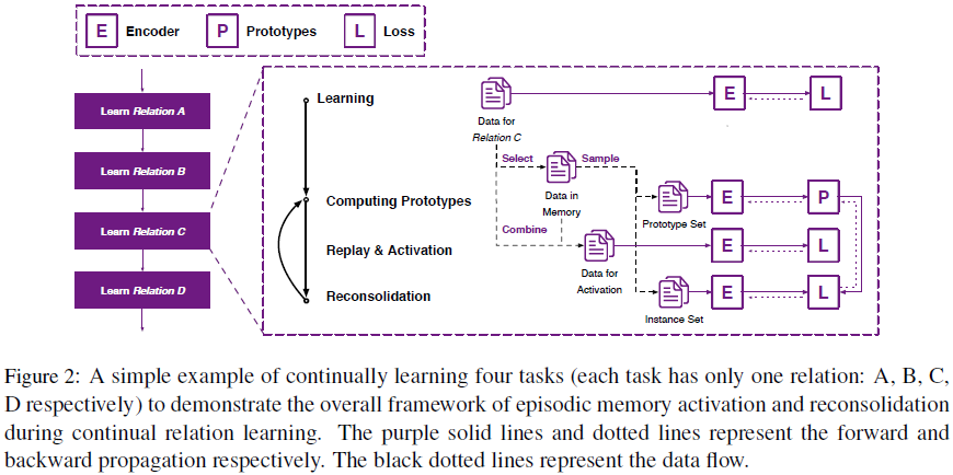
An example \(x\) is first tokenized into several tokens, then input into an example encoder to compute its corresponding embedding. Special tokens are added into the tokenized tokens to indicate the beginning and ending positions of entities related to the relations in sentences. The example encoding operation is denoted as \(\mathrm{x}=f(x)\), where \(\mathrm{x}\in\mathrm{\mathbb{R}}^d\) is the semantic embedding of \(x\), and \(d\) is the embedding dimension. A bidirectional long short-term memory (BiLSTM) network is selected as the example encoder in this paper, but other models, such as BERT, can also be adopted. When the \(k\)-th task is arising, the example encoder has not seen any examples of new relations before, and cannot properly encode their semantic features. Thus, the example encoder is first fine-tuned on \(\mathcal{T}_k=\{(x_1^{\mathcal{T}_k},y_1^{\mathcal{T}_k}),...,(x_N^{\mathcal{T}_k},y_N^{\mathcal{T}_k})\}\) to grasp new relation patterns in \(\mathcal{R}_k\). The loss function of learning the \(k\)-th task is as follows: \(\mathcal{L}(\theta)=-\sum\limits_{i=1}^N\sum\limits_{j=1}^{\vert\tilde{\mathcal{R}_k}\vert}\delta_{y_i^{\mathcal{T}_k}=r_j}\times\log\frac{\exp(g(f(x_i^{\mathcal{T}_k}),\mathrm{r}_j))}{\sum_{l=1}^{\vert\tilde{\mathcal{R}_k}\vert}\exp(g(f(x_i^{\mathcal{T}_k}),\mathrm{r}_l))}\), where \(\mathrm{r}_j\) is the embedding of the \(j\)-th relation \(r_j\in\tilde{\mathcal{R}_k}\) in the all known relation set \(\tilde{\mathcal{R}_k}\), \(g(\cdot,\cdot)\) is the function to compute similarities between embeddings (e.g., cosine similarity), and \(\theta\) is the parameters that can be optimized, including the example encoder parameters and relation embeddings. If \(y_i^{\mathcal{T}_k}=r_j\), \(\delta_{y_i^{\mathcal{T}_k}=r_j}=1\); otherwise, \(\delta_{y_i^{\mathcal{T}_k}=r_j}=0\). For each new relation, its embedding is first randomly initialized and then optimized by minimizing the loss above.
After several epochs of fine-tuning on the new task \(\mathcal{T}_k\), a few diverse examples from \(\mathcal{T}_k\) are selected and stored into the memory \(\mathcal{M}_k\). After encoding all examples of the \(k\)-th task \(\mathcal{T}_k\) into embeddings \(\{\mathrm{x}_1^{\mathcal{T}_k},...,\mathrm{x}_N^{\mathcal{T}_k}\}\), a K-Means clustering is conducted on the \(N\) example embeddings, where the number of clusters is the memory size \(B\). Then, for each cluster, the example closest to the cluster centroid is selected and its relation is recorded. The selected example set is denoted as \(\mathcal{C}_k\). By counting the example number in \(\mathcal{C}_k\) for each relation, the importance of a relation can be determined; the more selected examples a relation has, the more important it is. For more important relations, at least \(\lfloor\frac{B}{\vert\mathcal{R}_k\vert}\rfloor\) examples are selected. For less important relations, at most \(\lceil\frac{B}{\vert\mathcal{R}_k\vert}\rceil\) examples are selected. If a relation does not have enough examples to fill its allocated memory, this memory will be re-allocated for other relations. For each relation, a K-Means clustering is applied to its own examples and the number of clusters is its allocated example number in the memory. For each cluster, the example closest to the cluster centroid is selected and stored into the memory \(\mathcal{M}_k\).
The whole memory set \(\tilde{\mathcal{M}}_k=\bigcup_{i=1}^k\mathcal{M}_i\) is obtained by combining all examples in the episodic memory. To compute relation prototypes, for each known relation \(r_i\in\tilde{\mathcal{R}_k}\), a prototype set is sampled \(\mathcal{P}_i=\{x_1^{\mathcal{P}_i},...,x_{\vert\mathcal{P}_i\vert}^{\mathcal{P}_i}\}\), where each example \(x_i^{\mathcal{P}_i}\) comes from \(\tilde{\mathcal{M}}_k\) and its label equals \(r_i\), and its prototype embedding is computed as \(\mathrm{p}_i=\frac{\sum_{j=1}^{\vert\mathcal{P}_i\vert}f(x_j^{\mathcal{P}_i})}{\vert\mathcal{P}_i\vert}\), where \(\mathrm{p}_i\) is the relation prototype embedding of \(r_i\in\tilde{\mathcal{R}_k}\). In memory replay and activation, the whole memory set \(\tilde{\mathcal{M}}_k\) and the \(k\)-th training set \(\mathcal{T}_k\) will be combined into an activation set \(\mathcal{A}_k=\tilde{\mathcal{M}}_k\cup\mathcal{T}_k=\{(x_1^{\mathcal{A}_k},y_1^{\mathcal{A}_k}),...,(x_M^{\mathcal{A}_k},y_M^{\mathcal{A}_k})\}\) to continually activate models to learn new relations and remember old relations, where \(M\) is the total example number of both \(\tilde{\mathcal{M}}_k\) and \(\mathcal{T}_k\). The loss function is \(\mathcal{L}^{\mathcal{A}}(\theta)=-\sum\limits_{i=1}^M\sum\limits_{j=1}^{\vert\tilde{\mathcal{R}_k}\vert}\delta_{y_i^{\mathcal{A}_k}=r_j}\times\log\frac{\exp(g(f(x_i^{\mathcal{A}_k}),\mathrm{r}_j))}{\sum_{l=1}^{\vert\tilde{\mathcal{R}_k}\vert}\exp(g(f(x_i^{\mathcal{A}_k}),\mathrm{r}_l))}\).
Memory reconsolidation is the final learning step, targeting at better grasp of relation prototypes. For each known relation \(r_i\in\tilde{\mathcal{R}_k}\), an instance set \(\mathcal{I}_i=\{x_1^{\mathcal{I}_i},...,x_{\vert\mathcal{I}_i\vert}^{\mathcal{I}_i}\}\) is sampled similar to sampling prototype set \(\mathcal{P}_i\), where each example \(x_i^{\mathcal{I}_i}\in\mathcal{I}_i\) also comes from \(\tilde{\mathcal{M}}_k\) and its label equals \(r_i\). The loss function of the memory reconsolidation is \(\mathcal{L}^{\mathcal{R}}(\theta)=-\sum\limits_{i=1}^{\vert\tilde{\mathcal{R}_k}\vert}\sum\limits_{j=1}^{\vert\mathcal{I}_i\vert}\log\frac{\exp(g(f(x_j^{\mathcal{I}_i}),\mathrm{p}_i))}{\sum_{l=1}^{\vert\tilde{\mathcal{R}_k}\vert}\exp(g(f(x_j^{\mathcal{I}_i}),\mathrm{p}_l))}\), where \(\mathrm{p}_l\) is the relation prototype embedding of \(r_l\in\tilde{\mathcal{R}_k}\).
For training the \(k\)-th task, \(\mathcal{L}(\theta)\) is first used to optimize parameters for several epochs. Then, some examples are selected for the memory. Finally, computing relation prototype, optimizing parameters with \(\mathcal{L}^{\mathcal{A}}(\theta)\), and optimizing parameters with \(\mathcal{L}^{\mathcal{R}}(\theta)\) are conducted iteratively until convergence. After finishing the \(k\)-th task, for each known relation \(r_i\in\tilde{\mathcal{R}_k}\), all of its memorized examples \(\mathcal{E}_i=\{x_1^{\mathcal{E}_i},...,x_S^{\mathcal{E}_i}\}\) are collected from the whole memory \(\tilde{\mathcal{M}}_k\), where \(S\) is the example number of \(r_i\) in the memory, and final relation prototype for prediction is computed as \(\tilde{\mathrm{p}}_i=\frac{\mathrm{r}_i+\sum_{j=1}^S f(x_j^{\mathcal{E}_i})}{1+S}\), where \(\mathrm{r}_i\) is the relation embedding of \(r_i\). For each query example \(x\) in \(\tilde{\mathcal{Q}_k}\), its score function is defined for the relation \(r_i\) as \(s(x,r_i)=g(f(x),\tilde{\mathrm{p}}_i)\), where \(\tilde{\mathrm{p}}_i\) is the final prototype of the relation \(r_i\). Finally, the prediction \(y\) for the query \(x\) is calculated by: \(y=\arg\max\limits_{r_i\in\tilde{\mathcal{R}_k}}s(x,r_i)\).
Three benchmark datasets are used: (1) FewRel, containing 80 relations and 56,000 examples, is split into 10 clusters of relations for 10 tasks with each relation belongs to only one task. Each example in these tasks is associated with a relation and a candidate set of 10 randomly selected relations for evaluation. (2) SimpleQuestion (SimpleQ), containing 108,442 questions, each linked to a relation, is split into 20 clusters of relations to construct 20 tasks. (3) TACRED, containing 42 relations and 21,784 examples, is split into 10 clusters of relations to construct 10 tasks, and randomly sample candidate relation sets consisting of 10 relations for each example. Two evaluation settings are used: (1) whole performance, which calculates the accuracy on the whole test set of all tasks, and (2) average performance, which averages the accuracy on all seen tasks. As average performance highlights the performance of handling catastrophic problem; thus, it is the main metric to evaluate models. To compare with the then state-of-the-art continual relation learning model, EA-EMR[58], many settings (task sequence, hidden embedding dimension, pre-trained input embeddings, etc.) are consistent with theirs. Seven baseline models are compared: (1) Lower Bound, which continually fine-tunes models for each new task without memorizing any historical examples; (2) Upper Bound, which remembers all examples in history and continually re-train models with all data; (3) EWC (elastic weight consolidation), which uses Fisher information to measure the parameter importance to old tasks, and slows down the update of those parameters important to old tasks; (4) EMR, which memorizes a few historical examples and simply conducts memory replay; (5) GEM[51], which adds a constraint on directions of new gradients to make sure that optimization directions do not conflict with gradients on old tasks; (6) AGEM[52], which takes the gradient on sampled memorized examples from memory as the only constraint on the optimization directions of the current task; (7) EA-EMR[58], which introduces memory replay and embedding aligned mechanism to enhance previous tasks and mitigate the embedding distortion when trained on new tasks.
The results show that EMAR significantly outperforms other baselines (including the then SOTA EA-EMR) in almost all settings. On SimpleQ dataset, the performance of EMAR is on par with EA-EMR and EMR, probably because the SimpleQ benchmark is over simple. On FewRel and TACRED benchmarks, EMAR outperforms all the baseline models with a large margin, showing the superiority of the proposed episodic memory activation and reconsolidation mechanism. However, there is still a huge gap between EMAR and the upper bound. The average performance of models at each step show that (1) the performance of all the models decreases in some degree with increasing numbers of tasks, indicating that catastrophically forgetting old relations is inevitable; (2) the memory-based methods significantly outperform the consolidation-based method; (3) EMAR achieves a much better results compared to EA-EMR, showing the effectiveness of the memory reconsolidation and the importance of relation prototypes over rote memorization.
Memory size indicates the number of remembered examples for each task. Comparing three memory sizes, 10, 25, and 50, show that (1) with the increasing memory size, the performance of all models improves, indicating that the memory size is one of the key factors determining the performance of continual relation learning models; (2) on both FewRel and TACRED, EMAR keeps performing the best under different memory sizes, indicating that adopting relation prototypes is a more effective way to utilize memory compared with existing memory-based methods.
To show the effect of prototypes and reconsolidation, a case study is conducted to show the feature space changes at different training steps by EA-EMR and EMAR. The results show that the features learnt by EA-EMR become denser with increasing steps, thus harder to classify; but the features space of EMAR is more sparse and more distinguishable for classification. The \(L_2\) regularization used in EA-EMR for keeping the instance distribution of old relations leads to higher density in the feature space and smaller distances between different relations after several training steps. On the contrary, EMAR avoids forgetting previous relations by using relation prototypes for reconsolidation that allows EMAR to utilize larger feature spaces for representing examples and prototypes.
OML-ER and ANML-ER
OML-ER and ANML-ER[40] combine pre-trained BERT model with meta-learning and sparse memory (or experience) replay for lifelong text classification and relation extraction tasks. This study differs from Meta-MbPA in three aspects: (1) training examples to be written to memory are selected randomly by a probability, instead of using a diversity-based criterion; (2) there is no local adaptation in either training or testing stage; and (3) meta learning is formulated differently.
In the meta learning of Meta-MbPA, local adaptation is treated as the base task and representation learning as the meta task. By contrast, this paper adopts model agnostic meta-learning (MAML)[41] approach, where meta learning is to train a model on several related tasks such that it can transfer knowledge and adapt to new tasks using only a few examples. The goal of MAML is to learn to adapt quickly from the support set such that the model can perform well on the query set, where the support set refers to a few training examples for adaptation and the query set refers to a separate set of examples for evaluation. The key idea of MAML is to train a model’s initial parameters such that the model has maximal performance on a new task after the parameters have been updated through one or more gradient steps computed with a small amount of data from that new task.
During meta-training, a two-level optimization process is performed: an inner-loop performs task adaptation using the support set and an outer-loop performs meta-updates using the query set. In the inner loop, parameters \(\theta\) of the model \(f_{\theta}\) are updated to \(\theta_{i}^{\prime}\) for task \(\mathcal{T}_i\) by \(m\) steps of gradient-based update \(U\) on the support set as: \(\theta_{i}^{\prime}=U(\mathcal{L}_{\mathcal{T}_i}^s,\theta,\alpha,m)\) where \(\mathcal{L}_{\mathcal{T}_i}^s\) is the loss on the support set and \(\alpha\) is the inner-loop learning rate. In the outer-loop, the meta-objective is to have \(f_{\theta_{i}^{\prime}}\) generalize well across tasks from a distribution \(p(\mathcal{T})\): \(J(\theta)=\sum\limits_{\mathcal{T}_i\sim p(\mathcal{T})}\mathcal{L}_{\mathcal{T}_i}^q(f_{U(\mathcal{L}_{\mathcal{T}_i}^s,\theta,\alpha,m)})\) where \(\mathcal{L}_{\mathcal{T}_i}^q\) is the loss on the query set. The outer-loop optimization does the update with the outer-loop learning rate \(\beta\) as: \(\theta\leftarrow\theta -\beta\nabla_{\theta}\sum\limits_{\mathcal{T}_i\sim p(\mathcal{T})}\mathcal{L}_{\mathcal{T}_i}^q(f_{\theta_{i}^{\prime}})\). This involves computing second-order gradients, i.e., the backward pass works through the update step from \(\theta\) to \(\theta_{i}^{\prime}\), which is a computationally expensive process. A first-order approximation of MAML (FOMAML)[41] has been shown to perform nearly the same, where second derivatives are omitted and the gradients are computed with respect to \(\theta_{i}^{\prime}\) rather than \(\theta\). Thus, the outer-loop optimization step is reduced to: \(\theta\leftarrow\theta -\beta\sum\limits_{\mathcal{T}_i\sim p(\mathcal{T})}\nabla_{\theta_{i}^{\prime}}\mathcal{L}_{\mathcal{T}_i}^q(f_{\theta_{i}^{\prime}})\). During meta-testing, new tasks are learned from the support sets and the performance is evaluated on the corresponding query sets. During the inner-loop of an episode, the FOMAML setup performs one step of SGD on each of the \(m\) batches in the support set. Starting with parameters \(\theta_0=\theta\), it results in a sequence of parameters \(\theta_1,...,\theta_m\) using the losses \(\mathcal{L}^1,...,\mathcal{L}^m\). The meta-gradient computed on the query set of the episode is: \(g_{\mathrm{FOMAML}}=\frac{\partial\mathcal{L}^q(\theta_m)}{\partial\theta_m}\). Following the Taylor series approximation approach[42], the expected gradient under minibatch sampling could be expressed as: \(\mathrm{\mathbb{E}}[g_{\mathrm{FOMAML}}]=\mathrm{\mathbb{E}}\bigg[\frac{\partial\mathcal{L}^q(\theta_m)}{\partial\theta}-\frac{\alpha}{2}\frac{\partial}{\partial\theta}\bigg(\sum\limits_{j=1}^m\frac{\partial\mathcal{L}^j(\theta_{j-1})}{\partial\theta}\cdot\frac{\partial\mathcal{L}^q(\theta_m)}{\partial\theta}\bigg)\bigg]+O(\alpha^2)\) where \(\alpha\) is the inner-loop learning rate. Outer-loop gradient descent with this \(g_{\mathrm{FOMAML}}\) gradient approximately solves the following optimization problem: \(\min\limits_{\theta}\mathrm{\mathbb{E}}\bigg[\mathcal{L}^q(\theta_m)-\frac{\alpha}{2}\bigg(\sum\limits_{j=1}^m\frac{\partial\mathcal{L}^j(\theta_{j-1})}{\partial\theta}\cdot\frac{\partial\mathcal{L}^q(\theta_m)}{\partial\theta}\bigg)\bigg]\). This objective seeks to minimize the loss on the query set along with maximizing the dot product between the support and query set gradients. Thus, integrating previously seen examples into the query set in a FOMAML framework could also potentially improve continual learning by minimizing interference and maximizing transfer[43].
A continual learning consists of a stream of \(K\) tasks \(\mathcal{T}_1,\mathcal{T}_2,...,\mathcal{T}_K\). For supervised learning tasks, every task \(\mathcal{T}_i\) consists of a set of data points \(x_j\) with labels \(y_j\), \(\{(x_j,y_j)\}_{j=1}^{N_i}\) that are locally i.i.d., where \(N_i\) is the size of task \(\mathcal{T}_i\). The experiments make only one pass over the stream of tasks without identifiers of tasks. An episodic memory \(\mathcal{M}\) is maintained to store previously seen examples. Episodes for meta-training are constructed from the stream of examples as well as randomly sampled examples from \(\mathcal{M}\). A sparse experience replay is performed, which means a small number of examples are drawn from \(\mathcal{M}\) after seeing many examples from the stream. The structure of episodes and experience replay is illustrated in the Figure below. In regular episode, data points arrive in mini-batches of a given size \(b\) and every data point has a probability \(p_{write}\) of being written into \(\mathcal{M}\). Given a buffer size \(m\), episode \(i\) is constructed on-the-fly by taking \(m\) mini-batches from the stream as the support set \(\mathcal{S}_i\) and the next batch as the query set \(\mathcal{Q}_i\). The experience replay mechanism is defined as consisting of two fixed hyperparameters: (1) replay interval \(R_I\), which indicates the number of data points seen between two successive draws from memory, and (2) replay rate \(r\in[0,1]\), which indicates the proportion of examples to draw from memory relative to \(R_I\). Thus, after every \(R_I\) examples from the stream, \(\lfloor r\cdot R_I\rfloor\) examples are drawn from the memory and used as query set. To perform experience replay in an episodic fashion, the replay frequency \(R_F\) is computed as: \(R_F=\Big\lceil\frac{R_I/b+1}{m+1}\Big\rceil\). Hence, every \(R_F\) episodes, a random batch of size \(\lfloor r\cdot R_I\rfloor\) is drawn from \(\mathcal{M}\) as the query set. For regular episodes, the query set is obtained from the data stream. The support set for replay episodes is still constructed from the data stream. A high \(r\) and/or a low \(R_I\) ensures that information is not forgotten, but a low \(r\) and/or a high \(R_I\) ensures sparse replay and computational efficiency. During meta-testing, \(m\) batches are randomly drawn from the memory as the support set and the entire test set of the respective task is taken as the query set for evaluation.
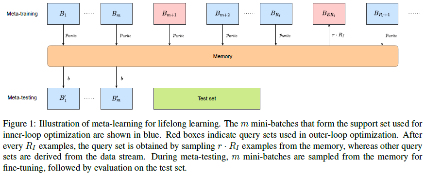
OML (Online aware Meta-learning)[44] is a meta-objective for minimizing interference in addition to maximizing fast adaptation for learning the Representation Learning Network (RLN). OML-ER extends OML by augmenting it with an episodic memory module to perform experience replay (ER). As illustrated in the Figure below, OML-ER model \(f_{\theta}\) is composed of two functions: a representation learning network (RLN) \(h_{\phi}\) with parameters \(\phi\) and a prediction learning network (PLN) \(g_W\) with parameters \(W\) such that \(\theta=\phi\cup W\) and \(f_{\theta}(x)=g_W(h_{\phi}(x))\) for an input \(x\). In each episode, the RLN is frozen while the PLN is fine-tuned during the inner-loop optimization. In the outer-loop, both the RLN and the PLN are meta-learned. During the inner-loop optimization in episode \(i\), the PLN is fine-tuned on the support set mini-batches \(\mathcal{S}_i\) with SGD to give: \(W_i^{\prime}=\mathrm{SGD}(\mathcal{L}_i,\phi,W,\mathcal{S}_i,\alpha)\) where \(\mathcal{L}_i\) is the loss function. Using the query set, the optimization objective is: \(J(\theta)=\mathcal{L}_i(\phi,W_i^{\prime},\mathcal{Q}_i)\). During a regular episode, the objective encourages generalization to unseen data whereas during a replay episode, it promotes retention of knowledge from previously seen data. For the outer-loop optimization, Adam optimizer is used with a learning rate \(\beta\) to update parameters of both RLN and PLN: \(\theta\leftarrow\mathrm{Adam}(J(\theta),\beta)\). The optimization uses the first-order variant where the gradients are taken with respect to \(\theta_i^{\prime}=\phi\cup W_i^{\prime}\). The RLN uses the output from the [CLS] token of a fully fine-tuned \(\mathrm{BERT}_{\mathrm{BASE}}\) and the PLN uses a single linear layer mapping to the classes.
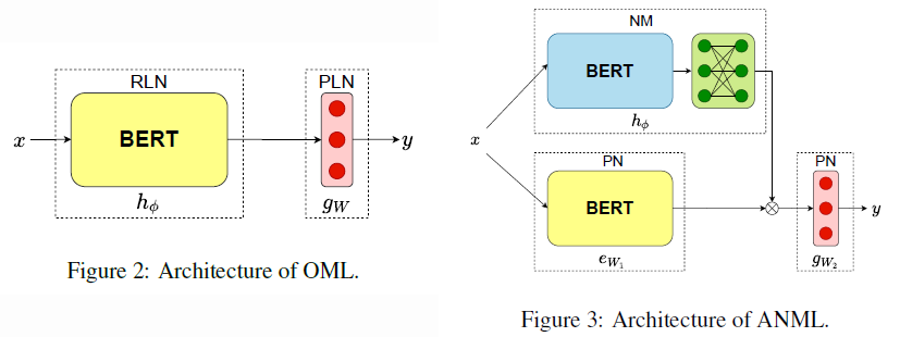
ANML (A Neuromodulated Meta-Learning Algorithm)[45] is composed of a neuromodulatory network (NM) and a regular prediction learning network (PN), where NM gates the forward pass of the PN and thus also indirectly controls the backward pass of (i.e. selective plasticity) the PN. The ANML differentiates through a sequential learning process to meta-learn an activation-gating function that enables context-dependent selective activation within a deep neural network. ANML-ER model \(f_{\theta}\) extends ANML by augmenting it with an episodic memory module to perform experience replay (ER). As illustrated in the Figure above, the NM is a function \(h_{\phi}\) with parameters \(\phi\), and the PN is a composite function \(g_{W_2}\circ e_{W_1}\) with parameters \(W=W_1\cup W_2\). The output is obtained as: \(f_{\theta}(x)=g_{W_2}(e_{W_1}\cdot h_{\phi}(x))\). In the inner-loop, the NM is fixed while the PN is fine-tuned on the support set, using the SGD function similar to OML-ER: \(W_i^{\prime}=\mathrm{SGD}(\mathcal{L}_i,\phi,W,\mathcal{S}_i,\alpha)\). In the outer-loop, both the NM and the PN are updated with first-order gradients as \(\theta\leftarrow\mathrm{Adam}(J(\theta),\beta)\). The PN is, as in OML-ER, the \(\mathrm{BERT}_{\mathrm{BASE}}\) encoder followed by a linear mapping to the classes. The NM uses \(\mathrm{BERT}_{\mathrm{BASE}}\) followed by two linear layers (768 units) with ReLU non-linearity between them and a final sigmoid non-linearity to limit the gating signal to [0, 1]. The NM BERT is frozen throughout to reduce the total number of parameters.
Four BERT-based baselines are used: (1) SEQ trains all tasks sequentially without replay; (2) REPLAY extends SEQ by sparse experience replay after seeing \(R_I\) examples from stream using \(\lfloor r\cdot R_I\rfloor\) random examples from memory; (3) A-GEM[52] modified by randomly sampling data points from the memory in sparse intervals; (4) MTL trains models for multiple epochs on mini-batches that are sampled i.i.d. from the pool of all tasks. The datasets for text classification are the same as those used in MbPA++ and Meta-MbPA. Relation extraction task uses a lifelong relation extraction benchmark based on the few-shot relation classification dataset FewRel that contains 80 relations and their corresponding names. Each training/testing sentence has a ground-truth relation as well as a set of 10 negative candidate relations. The goal is to predict the correct relation among them. To construct tasks for continual learning, they first perform K-means clustering over the average GloVe embeddings of the relation names to obtain 10 disjoint clusters. Each task then comprises of data points having ground-truth relations from the corresponding cluster. The evaluation metric is the accuracy on a single test set containing relations from all the clusters. For text classification, \(p_{write}=1\), replay 96 examples from memory for every 9,600 examples from stream, \(b=16\), \(r=0.01\), \(R_I=9600\), \(m=5\), input sequence length truncated to 300 for ANML-ER and 448 for all others. For relation extraction, sentence-relation pairs are concatenated with a [SEP] token between them to serve as the input; \(R_I=1600\), \(r=0.01\), \(b=4\), \(m=5\), and \(p_{write}=1\).
The text classification results show that OML-ER and ANML-ER substantially outperform SEQ, A-GEM, and REPLAY, but underperform MTL. Compared with previous studies, OML-ER and ANML-ER appear to outperform MbPA++, but underperform LAMOL and Meta-MbPA. There is no significant performance difference between OML-ER and ANML-ER. The relation extraction results show that OML-ER and ANML-ER significantly outperform SEQ, A-GEM, and REPLAY, but substantially underperform MTL. Compared with previous studies, OML-ER and ANML-ER appear to outperform the previous state-of-the-art LSTM-based method EMAR[46], despite it using task identities and training for multiple epochs. The differences between OML-ER and ANML-ER are not statistically significant.
Ablation studies show that experience replay is the most important component and meta-test fine-tuning plays a negligible role in both OML-ER and ANML-ER. Neuromodulation also plays insignificant role in ANML-ER. Even though OML-ER, ANML-ER and MAML-ER are equally successful in terms of performance, OML-ER is computationally more efficient as only its PLN (a single linear layer) is fine-tuned in the inner-loop.
Increasing replay rate from 1% to 4% significantly increases the performance of REPLAY and OML-ER models on both text classification and relation extraction, but the increased performance is still significantly below the performance of MTL. Decreasing the memory from storing all examples (\(p_{write}=1\)) to storing only 5% (\(p_{write}=0.05\)) or 1% (\(p_{write}=0.01\)) of the examples does not change the performance on text classification and only modestly reduces the performance on relation extraction.
In conclusion, OML-ER achieves both efficient training and efficient inference. Its training is fast because its inner-loop, which makes up a large portion of the training, involves only updating the small PLN. Its inference is fast because it relies only on a small number of updates on randomly drawn examples from memory. Furthermore, it also retains its performance when the memory capacity is scaled down.
ELLE
Qin et al. (2022)[47] address two challenges of efficient lifelong pre-training: (1) efficient knowledge growth. As knowledge accumulates from new tasks in lifelong learning, there is a need to increase model capacity to maintain learning efficiency. (2) proper knowledge stimulation. For a downstream task that requires knowledge primarily from a specific domain, there is a need to properly stimulate the domain-specific knowledge for the task. For the first challenge, ELLE adopts a function preserved model expansion method to flexibly expand the width and depth of an existing pre-trained language model (PLM). Before being adapted to a new domain, the expanded PLM performs a function recovering warmup, a form of memory replay, to regain the functionality of the original PLM. For the second challenge, ELLE pre-implants domain prompts during pre-training to prime the PLM with labels of the knowledge domains. During downstream fine-tuning, these implanted prompts stimulate the corresponding knowledge for specific downstream tasks. The experimental results using pre-trained BERT and GPT show the superiority of ELLE over multiple lifelong learning baselines in both pre-training efficiency and downstream task performances.
Given a series of tokens as an input \(\mathrm{x}=\{w_1,...,w_{\vert\mathrm{x}\vert}\}\) to a PLM \(\mathcal{M}\) with an embedding layer and \(L\) Transformer layers, \(\mathcal{M}\) first converts the input into embeddings \(\{\mathrm{h}_1^0,...,\mathrm{h}_{\vert\mathrm{x}\vert}^0\}\), which are then processed sequentially by each Transformer layer into contextualized hidden representations \(\mathrm{H}^l=\{\mathrm{h}_1^l,...,\mathrm{h}_{\vert\mathrm{x}\vert}^l\}\), where \(1\leq l\leq L\). The sequentially processed stream of corpora \(\bar{\mathcal{D}}_N\) from \(N\) domains is denoted as \(\bar{\mathcal{D}}_N=\{\mathcal{D}_1,...,\mathcal{D}_N\}\), where \(\mathcal{D}_i=\{\mathrm{x}_i^j\}_{j=1}^{\vert\mathcal{D}_i\vert}\). Given a PLM \(\mathcal{M}_1\) that has been well trained on \(\mathcal{D}_1\), for the \(i\)-th task (\(i>1\)), the goal is to continually pre-train the existing PLM \(\mathcal{M}_{i-1}\) to learn new knowledge on \(\mathcal{D}_i\) and obtain a new PLM \(\mathcal{M}_i\) that should not forget the previously learned knowledge of \(\bar{\mathcal{D}}_{i-1}\). As illustrated in the Figure below, given an existing PLM \(\mathcal{M}_{i-1}\) trained on previous data \(\bar{\mathcal{D}}_{i-1}\), the width and depth of \(\mathcal{M}_{i-1}\) is first expanded to construct an enlarged PLM \(\mathcal{M}_{i-1}^{\mathrm{WD}}\) to improve its training efficiency. Then, the \(\mathcal{M}_{i-1}^{\mathrm{WD}}\) is trained by performing function recovering warmup (FRW) to inherit the knowledge of \(\mathcal{M}_{i-1}\) to obtain \(\mathcal{M}_{i-1}^{\mathrm{WD}+}\). The two steps above are collectively named as function preserved model expansion. Then, \(\mathcal{M}_{i-1}^{\mathrm{WD}+}\) is continually pre-trained to gain new knowledge on \(\mathcal{D}_i\). To mitigate the catastrophic forgetting on the previously learned knowledge, data-based memory replay on a subset of previously gathered data \(\bar{\mathcal{D}}_{i-1}^{sub}=\{\mathcal{D}_1^{sub},...,\mathcal{D}_{i-1}^{sub}\}\) conserved in the memory, where \(\mathcal{D}_k^{sub}=\{x_k^1,...,x_k^B\}\in\mathcal{D}_k\ (1\leq k\leq i-1)\) and \(B\) is the constrained memory size for each domain. Domain prompts are implanted into PLMs during the entire training process to help disentangling the knowledge during pre-training and stimulating needed knowledge for downstream tasks.
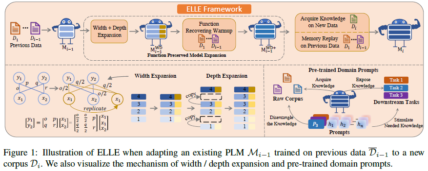
For width expansion, the function preserving initialization (FPI) from Chen et al. (2021)[48] is adopted to expand the matrices of all modules of a Transformer layer to arbitrary larger sizes and construct an enlarged PLM \(\mathcal{M}_{i-1}^{\mathrm{W}}\) that is initialized using the corresponding matrices of the original \(\mathcal{M}_{i-1}\) through parameter replication. As the example in the Figure above, the core principle of FPI is to divide the product of \(o\times x_1\) into multiple partitions, e.g. \(\frac{o}{2}\times x_1+\frac{o}{2}\times x_1\). Formally, FPI expands a matrix \(W\in\mathrm{\mathbb{R}}^{h_1\times h_2}\) of \(\mathcal{M}_{i-1}\) to an enlarged matrix \(W^{\prime}\in\mathrm{\mathbb{R}}^{(h_1+\Delta_{h_1})\times h_2}\) of \(\mathcal{M}_{i-1}^{\mathrm{W}}\) as follows: \(W_{(i,*)}^{\prime}=\frac{1}{C_i}\cdot W_{(m(i),*)}+\mathrm{\mathbb{I}}(C_i>1)\cdot\delta_i\) where \(C_i\) counts the number of partitions a specific neuron is split as \(C_i=\sum\limits_{i^{\prime}=1}^{h_1+\Delta_{h_1}}\mathrm{\mathbb{I}}(m(i^{\prime})=m(i))\); \(\mathrm{\mathbb{I}}(\cdot)\) is an indicator function; \(m(\cdot)\) denotes the mapping function between two matrices indexes as \(m(i)=i\) for \(i\in[1,h_1]\) and \(m(i)=U(\{1,...,h_1\})\) for \(i\in(h_1,h_1+\Delta_{h_1}]\) where \(U(\cdot)\) denotes a uniform sampling function; and \(\delta_i\in\mathrm{\mathbb{R}}^{h_2}\) is a random Gaussian noise. FPI aims to make the initialized targe model \(\mathcal{M}_{i-1}^{\mathrm{W}}\) having the same functionality as the source model \(\mathcal{M}_{i-1}\), which means that the two have approximately the same output given the same input. The random noise \(\delta_i\), newly introduced in this paper, aims to break the symmetry after the replication and accelerate later pre-training.
For depth expansion, this paper introduced a novel layer insertion method to construct a new PLM \(\mathcal{M}_{i-1}^{\mathrm{D}}\) with \(L+L^{\prime}\) layers, where \(1\leq L^{\prime}\leq L\). The \(L^{\prime}\) layers are randomly selected from \(\mathcal{M}_{i-1}\) and their parameters are copied to replication layers that are then inserted right before/after the corresponding original layers. At each expansion stage when new data comes, the layers that have not been copied before are chosen first. After width expansion and depth expansion, the enlarged model is denoted as \(\mathcal{M}_{i-1}^{\mathrm{WD}}\), which is expected to inherit \(\mathcal{M}_{i-1}\)’s knowledge contained in the parameters.
To ensure knowledge inheritance in the initialized target model \(\mathcal{M}_{i-1}^{\mathrm{WD}}\), it is pre-trained on the previous corpora \(\bar{\mathcal{D}}_{i-1}^{sub}\) conserved in the memory to recover the language abilities lost during model expansion, which is referred to as function recovering warmup (FRW). The model after FRW is denoted as \(\mathcal{M}_{i-1}^{\mathrm{WD}+}\).
To facilitate knowledge acquisition during pre-training, a soft prompt token as knowledge domain label is implanted into the input to prime the PLM. The prompt of domain \(i\) is a tunable vector \(\mathrm{p}_i\) that is prepended to the original token embeddings \(\mathrm{H}^0=\{\mathrm{h}_1^0,...,\mathrm{h}_{\vert\mathrm{x}\vert}^0\}\) for an input \(\mathrm{x}\in\mathcal{D}_i\). The resulting modified input \(\mathrm{H}^{0*}=\{\mathrm{p}_i;\mathrm{h}_1^0,...,\mathrm{h}_{\vert\mathrm{x}\vert}^0\}\) is then processed by all the Transformer layers. Each \(\mathrm{p}_i\) is optimized together with other parameters of the PLM during pre-training. During fine-tuning, the primed PLM is conditioned on these prompts by prepending a prompt to the input of downstream tasks. The most relevant domain prompt is manually decided for a specific downstream task.
Experiments are done with streaming data from 5 domains sequentially, i.e., the concatenation of (1) Wikipedia and BookCorpus (WB), (2) News Articles (NS), (3) Amazon Reviews (Rev), (4) Biomedical Papers (Bio), and (5) Computer Science Papers (CS). The quantity of data (about 3,400M tokens) for each corpus \(\mathcal{D}_i\) is comparable to the pre-training data of BERT. Because the cost of storage is far cheaper than the cost of computation for pre-training, a relatively large memory is used by randomly sampling 200M tokens (\(\mathcal{D}_i^{sub}\)) for each corpus \(\mathcal{D}_i\), which is about 6% of \(\mathcal{D}_i\) as opposed to about 1% in some earlier lifelong learning studies.
Both BERT and GPT are used in experiments with byte-level BPE vocabulary. The initial \(\mathcal{M}_1\) of 6 layers, hidden size of 384, 30M parameters, \(\mathrm{BERT}_{\mathrm{L6\_D384}}\)/\(\mathrm{GPT}_{\mathrm{L6\_D384}}\), is linearly enlarged 4 times to the final \(\mathcal{M}_5\) of 12 layers, hidden size of 768, 125M parameters, \(\mathrm{BERT}_{\mathrm{L12\_D768}}\)/\(\mathrm{GPT}_{\mathrm{L12\_D768}}\). Another set of experiments are done with larger model sizes from \(\mathrm{BERT}_{\mathrm{L12\_D768}}\) (125M) to \(\mathrm{BERT}_{\mathrm{L24\_D1024}}\) (355M). The number of training steps are 62,500, 5,000, and 20,000 for the \(\mathcal{M}_1\), the function recovering warmup, and learning new corpus with memory replay, respectively. For learning new corpus with memory replay, the sampling ratio of \(\mathcal{D}_i\) and \(\bar{\mathcal{D}}_{i-1}^{sub}\) is set to \(9:1\) in every batch. All the experiments are conducted under the same environment of 8 V100 GPUs with a batch size of 2,048 for the same training wall time at each training stage.
For pre-training evaluation, two metrics are used: (1) average perplexity (\(\mathrm{AP}\)) and (2) average increased perplexity (\(\mathrm{AP}^+\)). For a model checkpoint at time step \(T\) when learning the \(j\)-th domain, the checkpoint’s perplexity \(\mathrm{PPL}_{T,i}\) is measured on the validation set of each domain \(i\). Let \(\mathrm{PPL}_{i,i}^f\) be the perplexity on the \(i\)-th domain when the PLM finishes training on the \(i\)-th domain, the above metrics are calculated as follows: \(\mathrm{AP}=\exp(\frac{1}{j}\sum\limits_{i=1}^j\log\mathrm{PPL}_{T,i})\), \(\mathrm{AP}^+=\frac{1}{j-1}\sum\limits_{i=1}^{j-1}(\mathrm{PPL}_{T,i}-\mathrm{PPL}_{i,i}^f)\), where \(\mathrm{AP}\) measures the average performance on all the seen data \(\{\mathcal{D}_1,...,\mathcal{D}_j\}\), and \(\mathrm{AP}^+\) measures the influence of current data \(\mathcal{D}_j\) on previous data \(\bar{\mathcal{D}}_{j-1}\). Lower \(\mathrm{AP}\) indicates that the PLM generally learns more knowledge from existing domains, and lower \(\mathrm{AP}^+\) means that PLMs forget less knowledge learned before. For downstream task evaluation, a representative task is selected for fine-tuning PLMs on downstream tasks of each domain: Multi-Genre Natural Language Inference (MNLI) for WB, Hyperpartisan News Detection for NS, Helpfulness of a review for Rev, ChemProt for Bio, and ACL Anthology Reference Corpus (ARC) for CS.
The following 7 baseline models are used for comparison: (1) Naive. PLMs continually adapt to each domain. (2) EWC (Elastic Weight Consolidation)[54] uses \(L_2\) regularization on parameter changes. (3) MAS (Memory Aware Synapses)[53] estimates parameter importance via the gradients of the model outputs. (4) ER (Experience Replay) alleviates forgetting by jointly training models on a mixture of samples from new data \(\mathcal{D}_i\) and the memory \(\bar{\mathcal{D}}_{i-1}^{sub}\) with ratio of \(9:1\) in every batch. (5) A-GEM (Average Gradient Episodic Memory)[52] constrains the new parameter gradients to make sure that optimization directions do not conflict with gradients on old domains. (6) Logit-KD prevents forgetting by distilling knowledge from the previous model \(\mathcal{M}_{i-1}\) using the old data in the memory. (7) PNN (Progressive Neural Network) fixes the old PLM \(\mathcal{M}_{i-1}\) to completely avoid knowledge forgetting and grows new network with lateral connections for learning new knowledge.
The experimental results show superior performance of ELLE: (1) Compared with all the baselines, ELLE achieves the lowest \(\mathrm{AP}\) and second lowest \(\mathrm{AP}^+\) (2nd to PNN) after finishing training on each domain, demonstrating that ELLE can simultaneously acquire more new knowledge and mitigate forgetting old knowledge. (2) As pre-training progresses, the \(\mathrm{AP}\) of ELLE descends the fastest, showing the superior training efficiency of ELLE over all baselines. (3) ELLE performs the best on all downstream tasks, indicating that the knowledge learned during pre-training could be properly stimulated and leveraged for each downstream task. (4) The superiority of ELLE on \(\mathrm{BERT}_{\mathrm{L12\_D768}}\) is consistently observed on the larger model size, \(\mathrm{BERT}_{\mathrm{L24\_D1024}}\), and other model architectures, \(\mathrm{GPT}_{\mathrm{L12\_D768}}\). This shows that ELLE is agnostic to both the model size and the specific PLM model architecture.
The performance of the baseline models is in the following order: (1) Consolidation-based methods (EWC and MAS) perform on par with the naive baseline in either pre-training or downstream tasks, indicating that parameter regularization offers limited benefit for PLM’s knowledge acquisition. (2) Among memory-based methods, gradient-based replay (A-GEM) substantially underperforms data-based replay (ER and Logit-KD) in pre-training. On \(\mathrm{AP}\) and \(\mathrm{AP}^+\), A-GEM performs on par with the naive baseline, but ER and Logit-KD substantially outperform the naive baseline, demonstrating that replaying real data points (as opposed to weight gradients) could more efficiently learn new knowledge and mitigate the old knowledge forgetting problem. On the contrary, on downstream tasks, all of the memory-based methods perform comparable or worse than the naive baseline. (3) PNN achieves significantly lower \(\mathrm{AP}\) than non-progressive baselines, and is immune to knowledge forgetting (\(\mathrm{AP}^+=0\)). It also performs better on the downstream tasks than other baselines. This indicates that enlarging the network is an effective way for lifelong pre-training and also benefits downstream tasks.
Comparing width only expansion (WE+FRW), depth only expansion (DE+FRW), and both width and depth expansion (WE+DE+FRW) shows that: (1) All three achieve better pre-training and downstream performance than the non-expanding baseline, showing that increasing model size on each new task increases sample efficiency and training efficiency. (2) Expanding both width and depth is more efficient and performs better on downstream tasks (except NS) than expanding only width or depth. Only expanding depth will make the training process unstable.
Comparing expansion with and without FRW, i.e., WE+DE vs WE+DE+FRW, under the same wall time causes WE+DE to be trained for more steps. However, the results show that WE+DE achieves worse \(\mathrm{AP}\) and \(\mathrm{AP}^+\), indicating that without FRW, PLM would learn new knowledge slower and also forget more previous knowledge. As training progresses, \(\mathrm{AP}\) and \(\mathrm{AP}^+\) decrease faster with FRW, demonstrating that FRW can better recover the knowledge lost resulted from model expansion. WE+DE+FRW also performs slightly better than WE+DE in most of the downstream tasks, except the NS domain.
Comparing the model performance with and without random noise added to the newly copied parameters after width expansion, i.e., WE+DE+FRW and WE+DE+FRW+\(\delta_N\), shows that the added noises significantly speed up pre-training and improve overall downstream performance. This validates the hypothesis that random noises are useful for breaking the symmetry of the copied parameters, thus providing a better initialization favorable for further optimization.
Comparing the performance with and without pre-trained domain prompts, i.e., WE+DE+FRW+\(\delta_N\) and WE+DE+FRW+\(\delta_N\)+PT, shows that when aided with domain prompts, PLMs achieve lower \(\mathrm{AP}\) and \(\mathrm{AP}^+\) during pre-training, showing that domain prompts could accelerate pre-training and alleviate catastrophic forgetting. Furthermore, domain prompts generally improve downstream performance by stimulating the proper knowledge needed for each task. Comparing downstream performance without prompt and with wrong prompt prepended in the input, i.e., \(\mathrm{ELLE-PT}_{\mathrm{fine-tune}}\) and \(\mathrm{ELLE+\neg PT}_{\mathrm{fine-tune}}\), shows that both strategies have lower downstream performance than prepending the right prompt (ELLE). The lower performance of \(\mathrm{ELLE-PT}_{\mathrm{fine-tune}}\) can be attributed to a great gap between the formats of input during pre-training and fine-tuning. The lower performance of \(\mathrm{ELLE+\neg PT}_{\mathrm{fine-tune}}\) can be attributed to failure of stimulation of relevant knowledge by the wrong prompt.
Visualization of the attention patterns of different attention heads in a stream of PLMs (\(\{\mathcal{M}_1,...,\mathcal{M}_5\}\)) trained by ELLE shows similar patterns between a descendant PLM and its ancestor PLMs, even after the descendant PLM is further trained on new data and enlarged several times. This indicates that the expanded PLM by ELLE successfully inherits the knowledge from its “ancestor”, and thus exhibits similar functionality to some extent.
Implicit Memory Replay
In addition to retrieving actual training examples, or their encoded representations, of previously learned tasks from episodic memory for replay, some studies generate “pseudo examples” from the model to be trained for a new task and mixed them with the training examples of the new task for replaying/training. The pseudo examples reflect implicit memory of model weights that store generalized <context, next token> relations in the corpora of previous tasks. Thus, such generative replay can be referred to as implicit memory replay. The advantages of this category of approach include: (1) there is no need for extra memory or model capacity; and (2) it does not need to know the number of tasks in advance. Sun et al. (2019)[49] introduce LAMOL (LAnguage MOdeling for Lifelong Language Learning) that uses pre-trained GPT-2 as the initial language model and generates pseudo examples of previous tasks to be replayed in learning subsequent tasks. LAMOL outperforms MbPA++ but underperforms Meta-MbPA[40].
LAMOL
Many NLP tasks can be formulated as question answering (QA) tasks that can be addressed with a single model by training a language model (LM) that generates an answer based on the context and the question. Sun et al. (2019)[49] apply such LM to lifelong language learning (LLL) problem by simultaneously training it to generate either answers to given context-questions or pseudo examples (each containing context, question, and answer) to given generation tokens. The model, referred to as LAMOL, plays a dual role of both LM and QA model. During LLL, these pseudo old examples are trained with new examples from new tasks to help mitigate catastrophic forgetting. The input data format depends on the training objective. When training as a QA model, the LM learns to decode the answer after reading the context and question. When training as an LM, the LM learns to decode all three parts, context, question, and answer, given a generation token. Three special tokens are added, as illustrated in the Figure below: ANS is inserted between question and answer. During inference, the ANS signals the start of decoding for an answer. EOS is added as the last token of every example. Decoding stops when EOS is encountered. GEN is added as the first token during pseudo example generation to signal the start of decoding.
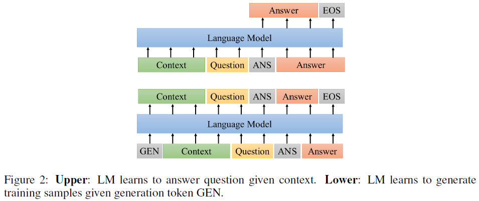
For a stream of, possibly unknown number of, tasks \(\{T_1,T_2,...\}\), before beginning training on each new task \(T_i\), \(i>1\), the model first generates pseudo examples \(T_i^{\prime}\) by top-\(k\) sampling that represent the data distribution of previous tasks \(T_1\),…,\(T_{i-1}\). Then, the LM trains on the mixture of \(T_i\) and \(T_i^{\prime}\). To balance the ratio between \(\vert T_i\vert\) and \(\vert T_i^{\prime}\vert\), the LM generates \(\gamma\vert T_i\vert\) pseudo examples, where \(\vert T_i\vert\) denotes the number of examples in task \(T_i\) and \(\gamma\) is the sampling ratio. If a generated example does not have exactly one ANS in it, then the example is discarded, which happens in only \(0.5\%\)~\(1\%\) of generated examples. During training, each example is formatted into both the QA format and the LM format. Then, in the same optimization step, both formats are fed into the LM to minimize the QA loss \(L_{QA}\) and LM loss \(L_{LM}\) together. Overall, the loss is \(L=L_{QA}+\lambda L_{LM}\), where \(\lambda\) is the weight of the LM loss.
Using the same GEN token for all tasks will cause a distant past task to contribute much less than immediate past task in generated pseudo examples, which may not be optimal for subsequent learning. To mitigate this, the GEN token is replaced with a task-specific token for each task to inform the model to generate pseudo examples belonging to the specific task. Under this setup, all previous tasks have the same share of the \(\gamma\vert T_i\vert\) generated pseudo examples, which is \(\frac{\gamma}{i-1}\vert T_i\vert\) for each of the previous \(i-1\) tasks. Two sets of tasks are used in this study: 5 disparate tasks and corresponding datasets (question answering-SQuAD, semantic parsing-WikiSQL, sentiment analysis-SST, semantic role labeling-QA-SRL, and goal-oriented dialogue-WOZ) mentioned in decaNLP[50], and 5 datasets (AGNews, Amazon, DBPedia, Yahoo, and Yelp) for text classification tasks used by MbPA++[36]. Evaluation metrics include: normalized F1 (nF1) for question answering and semantic role labeling, exact match (EM) for sentiment analysis and all text classification tasks, exact match of logical forms (lfEM) for semantic parsing, and turn-based dialogue state exact match (dsEM) for goal-oriented dialogue.
All methods use the smallest pre-trained GPT-2 model as the LM. Each task is trained for 9 epochs; greedy decoding is applied during inference. The following approaches are compared: (1) LAMOL In all experiments, \(k=20\) in top-\(k\) sampling and \(\lambda=0.25\) for weight of the LM loss. If the same GEN token is used for all tasks, it is denoted as \(\mathrm{LAMOL}_{\mathrm{GEN}}^{\gamma}\), where \(\gamma\) is the sampling ratio. If task-specific tokens are used, it is denoted as \(\mathrm{LAMOL}_{\mathrm{TASK}}^{\gamma}\). (2) Keep real data Pseudo examples are replaced by real examples from previous tasks. The number of real examples is equally split between previous tasks. This real example replay, denoted as \(\mathrm{LAMOL}_{\mathrm{REAL}}^{\gamma}\), can be considered as the upper bound of LAMOL. (3) Fine-tune The model is directly fine-tuned on the stream of tasks, one after another. This approach does not have LM loss; it only has QA loss. Note that fine-tune is not the same as the LAMOL with \(\gamma=0\), whose LM loss is still optimized. (4) Multitask learning All tasks are trained simultaneously, which is considered as the upper bound of lifelong learning. This can also be used to determine whether forgetting is caused by a lack of model capacity. (5) Regularization-based methods Online EWC[54] and MAS[53] are compared. (6) Gradient Episodic Memory (GEM)[51] When training each task, data from previous task are randomly sampled to the amount equivalent to 5% of the current task size and written into an episodic memory. In each optimization step, the GEM approach retrieves all the data in the memory to calculate the gradients for the previous tasks. (7) Improved memory-based parameter adaptation (MBPA++)[36] This paper re-implements the original paper and reports better scores using different hyperparameters.
The single task performance of GPT-2 on each of the 10 datasets are evaluated by training the model on GPT-2 independently. Comparing the results with their counterparts in the two papers, decaNLP and MbPA++, shows that the GPT-2 model outperforms the BERT-based model on text classification datasets by a large margin.
The effect of task order is evaluated on three small datasets: SST, QA-SRL, and WOZ. Six permutations of their order are used to train six of the seven approaches excluding the multitask learning that is considered as an upper bound and trained on the three datasets simultaneously. The final score for each order is obtained by evaluating the model at the end of training all three datasets. The average and standard deviation of the six scores of each method are compared. The results show that fine-tuned, EWC, MAS, GEM, and LAMOL with \(\gamma=0\) (\(\mathrm{LAMOL}_{\mathrm{GEN}}^0\), \(\mathrm{LAMOL}_{\mathrm{TASK}}^0\)) perform similarly and are much worse than LAMOL with \(\gamma>0\). The best performing method, \(\mathrm{LAMOL}_{\mathrm{GEN}}^{0.2}\), is only 1.8% below multitasked, suggesting little forgetting during LLL. When using LAMOL, the performance of old tasks maintains at almost the same level throughout the training process. When the sampling ratio is increased, the performance also increases, especially when increased from 0 to 0.05. A smaller standard deviation implies that it is affected less by task order. Adding task-specific tokens, i.e., comparing \(\mathrm{LAMOL}_{\mathrm{TASK}}^{\gamma}\) to \(\mathrm{LAMOL}_{\mathrm{GEN}}^{\gamma}\), reduces standard deviation and thus has a stabilizing effect.
The five decaNLP tasks are trained sequentially only in the order from large to small tasks: SQuAD, WikiSQL, SST, QA-SRL, and WOZ. LAMOL outperforms all baselines by a large margin and on average approaches within 2–3% of the multitasked upper bound. Also, the performance of LAMOL improves as the sampling ratio \(\gamma\) increases and task-specific tokens are used. There is a performance gap between \(\mathrm{LAMOL}_{\mathrm{TASK}}^{\gamma}\) and \(\mathrm{LAMOL}_{\mathrm{REAL}}^{\gamma}\). Using real examples is much more sample-efficient, as 5% of real examples beats 20% of pseudo-examples. This may be due to the less-than-ideal quality of the pseudo examples. The longer the paragraphs are, the harder it is for the model to create high-quality examples. Comparing the test scores of each method on each task throughout the sequential training reveals that LAMOL remembers previously learned knowledge nearly perfectly. Training SQuAD before training QA-SRL already gave QA-SRL a score around 40. Training QA-SRL, after SQuAD has been forgotten by WikiSQL ans SST trainings, recovers SQuAD score for fine-tune and MAS. These two facts suggest that SQuAD and SRL are similar tasks and that positive knowledge transfer may occur between them. If forward transfer exists, replaying pseudo examples also retains the forward transfer, as LAMOL can prevent QA-SRL score from being reduced by WikiSQL and SST training.
The performance of LLL on the five text classification datasets are compared between \(\mathrm{LAMOL}_{\mathrm{TASK}}^{0.2}\) and MbPA++ (both the original paper and the re-implementation by the LAMOL authors). The \(\mathrm{LAMOL}_{\mathrm{TASK}}^{0.2}\) significantly outperforms both versions of MbPA++.
The influence of sampling ratio \(\gamma\) is studied by training \(\mathrm{LAMOL}_{\mathrm{TASK}}^{\gamma}\) and \(\mathrm{LAMOL}_{\mathrm{GEN}}^{\gamma}\) for \(\gamma\in\{0.01, 0.03, 0.1, 0.3, 1.0\}\) on four tasks in the order: WikiSQL, SST, QA-SRL, and WOZ. With smaller \(\gamma\), the models are more likely to forget how to generate previous tasks. Models using task-specific tokens mitigate this somewhat. With larger \(\gamma\), the models have better overall performance. However, the gain appears to reaches plateau when \(\gamma\) is around 0.1 to 0.3.
Codes
- Nearest Neighbor Language Models (kNN-LM)
- Product-Key Memory Layers (PKM)
- Infinite-former
- Sparse and Continuous Attention Mechanisms
- Query-Key Normalization for Transformers
- FAISS, a library for efficient similarity search and clustering of dense vectors.
- ScaNN (Scalable Nearest Neighbors), a method for efficient vector similarity search at scale.
- Adaptive Softmax, an efficient softmax approximation for graphical processing units (GPU).
- Stanford Open Information Extraction
- Stanford Named Entity Recognizer
- JAX is a numerical computing library that combines NumPy, automatic differentiation, and first-class GPU/TPU support.
- Haiku is a simple neural network library for JAX that enables users to use object-oriented programming models while allowing full access to JAX’s pure function transformations.
- Moses, a statistical machine translation system
- Hopfield Networks
- Meta-Learning with Sparse Experience Replay
- Online-aware Meta-learning (OML)
- A Neuromodulated Meta-Learning Algorithm (ANML)
- Efficient Lifelong Pre-training for Emerging Data (ELLE)
- LAMOL: LAnguage MOdeling for Lifelong Language Learning
- A-GEM: Averaged Gradient Episodic Memory
- A re-implementation of MbPA++
- Episodic Memory Activation and Reconsolidation (EMAR)
- Sentence Embedding Alignment for Lifelong Relation Extraction (EMR & EA-EMR)
References
[1] Squire, L. R. and Zola, S. M. (1996) Structure and function of declarative and nondeclarative memory systems. Proc. Natl. Acad. Sci. USA, Vol. 93, pp. 13515–13522
[2] McGaugh, J. L. (2000) Memory–a Century of Consolidation. Science, Vol. 287(5451), pp. 248-51
[3] von Neumann, J. (1945) First Draft of a Report on the EDVAC. IEEE Ann. Hist. Comput., Vol. 15, No. 4, pp. 27–75
[4] Tay, Y., Tran, V. Q., Dehghani, M., Ni, J., Bahri, D., et al. (2022) Transformer Memory as a Differentiable Search Index. arXiv preprint arXiv:2202.06991
[5] Kaplan, J., McCandlish, S., Henighan, T., Brown, T. B., Chess, B., et al. (2020) Scaling Laws for Neural Language Models. arXiv preprint arXiv:2001.08361
[6] Abnar, S., Dehghani, M., Neyshabur, B., and Sedghi, H. (2021) Exploring the Limits of Large Scale Pre-training. arXiv preprint arXiv:2110.02095
[7] Tay, Y., Dehghani, M., Rao, J., Fedus, W., Abnar, S, et al. (2021) Scale Efficiently: Insights from Pre-training and Fine-tuning Transformers. arXiv preprint arXiv:2109.10686
[8] Lepikhin, D., Lee, H., Xu, Y., Chen, D., Firat, O., et al. (2020) GShard: Scaling Giant Models with Conditional Computation and Automatic Sharding. arXiv preprint arXiv:2006.16668
[9] Fedus, W., Zoph, B., and Shazeer, N. (2021) Switch Transformers: Scaling to Trillion Parameter Models with Simple and Efficient Sparsity. arXiv preprint arXiv:2101.03961
[10] Du, N., Huang, Y., Dai, A. M., Tong, S., Lepikhin, D., et al. (2021) GLaM: Efficient Scaling of Language Models with Mixture-of-Experts. arXiv preprint arXiv:2112.06905
[11] Graves, A., Wayne, G., Reynolds, M., Harley, T., Danihelka, I., et al. (2016) Hybrid computing using a neural network with dynamic external memory. Nature, Vol. 538, pp. 471–476
[12] Yogatama, D., de Masson d’Autume, C., and Kong, L. (2021) Adaptive Semiparametric Language Models. arXiv preprint arXiv:2102.02557
[13] Khandelwal, U., Levy, O., Jurafsky, D., Zettlemoyer, L., and Lewis, M. (2019) Generalization through Memorization: Nearest Neighbor Language Models. arXiv preprint arXiv:1911.00172
[14] Lample, G., Sablayrolles, A., Ranzato, M., Denoyer, L., and J\(\acute e\)gou, H. (2019) Large Memory Layers with Product Keys. arXiv preprint arXiv:1907.05242
[15] Burtsev, M. S., Kuratov, Y., Peganov, A., and Sapunov, G. V. (2020) Memory Transformer. arXiv preprint arXiv:2006.11527
[16] Wu, Q., Lan, Z., Gu, J., and Yu, Z. (2020) Memformer: The Memory-Augmented Transformer. arXiv preprint arXiv:2010.06891
[17] Wu, Y., Rabe, M. N., Hutchins, D., and Szegedy, C. (2022) Memorizing Transformers. arXiv preprint arXiv:2203.08913
[18] Zhang, Y. and Cai, D. (2022) Linearizing Transformer with Key-Value Memory Bank. arXiv preprint arXiv:2203.12644
[19] Katharopoulos, A., Vyas, A., Pappas, N., and Fleuret, F. (2020) Transformers are RNNs: Fast Autoregressive Transformers with Linear Attention. arXiv preprint arXiv:2006.16236
[20] Peng, H., Pappas, N., Yogatama, D., Schwartz, R., Smith, N. A., and Kong, L. (2021) Random Feature Attention. In Proc. of ICLR.
[21] Kasai, J., Peng, H., Zhang, Y., Yogatama, D., Ilharco, G., et al. (2021) Finetuning Pretrained Transformers into RNNs. arXiv preprint arXiv:2103.13076
[22] Martins, P. H., Marinho, Z., and Martins, A. F. T. (2021) \(\infty\)-former: Infinite Memory Transformer. arXiv preprint arXiv:2109.00301
[23] Martins, A. F. T., Farinhas, A., Treviso, M., Niculae, V., Aguiar, P. M. Q., and Figueiredo, M. A. T. (2020) Sparse and Continuous Attention Mechanisms. arXiv preprint arXiv:2006.07214
[24] Ramsauer, H., Schäfl, B., Lehner, J., Seidl, P., Widrich, M., et al. (2020) Hopfield Networks is All You Need. arXiv preprint arXiv:2008.02217
[25] Hochreiter, S. and Schmidhuber, J. (1997) Long Short-Term Memory. Neural Computation 9(8): 1735–1780
[26] Graves, A., Wayne, G., and Danihelka, I. (2014) Neural Turing Machines. arXiv preprint arXiv:1410.5401
[27] Weston, J., Chopra, S., and Bordes, A. (2014) Memory Networks. arXiv preprint arXiv:1410.3916
[28] Sukhbaatar, S., Szlam, A., Weston, J., and Fergus, R. (2015) End-To-End Memory Networks. Advances in neural information processing systems, 28.
[29] Rae, J. W., Hunt, J. J., Harley, I., Senior, A., Wayne, G., Graves, A., Lillicrap, T. P. (2016) Scaling Memory-Augmented Neural Networks with Sparse Reads and Writes. Advances in Neural Information Processing Systems, 29.
[30] Gulcehre, C., Chandar, S., Cho, K., and Bengio, Y. (2016) Dynamic Neural Turing Machine with Continuous and Discrete Addressing Schemes. arXiv preprint arXiv:1607.00036
[31] Gulcehre, C., Chandar, S., and Bengio, Y. (2017) Memory Augmented Neural Networks with Wormhole Connections. arXiv preprint arXiv:1701.08718
[32] McCloskey, M. and Cohen, N. (1989) Catastrophic interference in connectionist networks: The sequential learning problem. In: Psychology of Learning and Motivation, Vol. 24, pp. 109–165
[33] French, R. M. (1999) Catastrophic Forgetting in Connectionist Networks: Causes, Consequences and Solutions. In: Trends in Cognitive Sciences, 3(4), 128-135
[34] Ermis, B., Zappella, G., Wistuba, M., and Archambeau, C. (2022) Memory Efficient Continual Learning for Neural Text Classification. arXiv preprint arXiv:2203.04640
[35] Sprechmann, P., Jayakumar, S. M., Rae, J. W., Pritzel, A., Badia, A. P., et al. (2018) Memory-based Parameter Adaptation. arXiv preprint arXiv:1802.10542
[36] de Masson d’Autume, C., Ruder, S., Kong, L., and Yogatama, D. (2019) Episodic Memory in Lifelong Language Learning. arXiv preprint arXiv:1906.01076
[37] Wang, Z., Mehta, S. V., P´oczos, B., and Carbonell, J. (2020) Efficient Meta Lifelong-Learning with Limited Memory. arXiv preprint arXiv:2010.02500
[38] Clayton, N. S., Salwiczek, L. H., and Dickinson, A. (2007) Episodic memory. Current Biology, 17(6): R189–91
[39] Knoblauch, J., Husain, H., and Diethe, T. (2020) Optimal Continual Learning has Perfect Memory and is NP-HARD. arXiv preprint arXiv:2006.05188
[40] Holla, N., Mishra, P., Yannakoudakis, H., and Shutova, E. (2020) Meta-Learning with Sparse Experience Replay for Lifelong Language Learning. arXiv preprint arXiv:2009.04891
[41] Finn, C., Abbeel, P., and Levine, S. (2017) Model-Agnostic Meta-Learning for Fast Adaptation of Deep Networks. In: Proceedings of the 34th International Conference on Machine Learning, PMLR 70:1126-1135
[42] Nichol, A., Achiam, J., and Schulman, J. (2018) On First-Order Meta-Learning Algorithms. arXiv preprint arXiv:1803.02999
[43] Riemer, M., Cases, I., Ajemian, R., Liu, M., Rish, I., Tu, Y., and Tesauro, G. (2019) Learning to Learn without Forgetting by Maximizing Transfer and Minimizing Interference. In: International Conference on Learning Representations
[44] Javed, K. and White, M. (2019) Meta-Learning Representations for Continual Learning. arXiv preprint arXiv:1905.12588
[45] Beaulieu, S., Frati, L., Miconi, T., Lehman, J., Stanley, K. O., Clune, J., and Cheney, N. (2020) Learning to Continually Learn. arXiv preprint arXiv:2002.09571
[46] Han, X., Dai, Y., Gao, T., Lin, Y., Liu, Z., Li, P., Sun, M., and Zhou, J. (2020) Continual Relation Learning via Episodic Memory Activation and Reconsolidation. In: Proceedings of the 58th Annual Meeting of the Association for Computational Linguistics, pp. 6429–6440
[47] Qin, Y., Zhang, J., Lin, Y., Liu, Z., Li, P., Sun, M., Zhou, J. (2022) ELLE: Efficient Lifelong Pre-training for Emerging Data. arXiv preprint arXiv:2203.06311
[48] Chen, C., Yin, Y., Shang, L., Jiang, X., Qin, Y., Wang, F., Wang, Z., Chen, X., Liu, Z., and Liu, Q. (2021) bert2BERT: Towards Reusable Pretrained Language Models. arXiv preprint arXiv:2110.07143
[49] Sun, F.-K., Ho, C.-H., and Lee, H.-Y. (2019) LAMOL: LAnguage MOdeling for Lifelong Language Learning. In: International Conference on Learning Representations
[50] McCann, B., Keskar, N. S., Xiong, C., and Socher, R. (2018) The Natural Language Decathlon: Multitask Learning as Question Answering. arXiv preprint arXiv:1806.08730
[51] Lopez-Paz, D. and Ranzato, M. (2017) Gradient Episodic Memory for Continual Learning. arXiv preprint arXiv:1706.08840
[52] Chaudhry, A., Ranzato, M., Rohrbach, M., and Elhoseiny, M. (2018) Efficient Lifelong Learning with A-GEM. arXiv preprint arXiv:1812.00420
[53] Aljundi, R., Babiloni, F., Elhoseiny, M., Rohrbach, M., and Tuytelaars, T. (2017) Memory Aware Synapses: Learning what (not) to forget. arXiv preprint arXiv:1711.09601
[54] Schwarz, J., Luketina, J., Czarnecki, W. M., Grabska-Barwinska, A., Teh, Y. W., Pascanu, R., and Hadsell, R. (2018) Progress & Compress: A scalable framework for continual learning. arXiv preprint arXiv:1805.06370
[55] Cowan, N. (2008) What are the differences between long-term, short-term, and working memory? Progress in Brain Research, Vol. 169, pp 323-338
[56] Baddeley, A. (2010) Working memory. Current Biology, 20(4): R136-R140
[57] Alberini, C. M. (2005) Mechanisms of memory stabilization: are consolidation and reconsolidation similar or distinct processes? Trends in Neurosciences, 28(1): 51–56
[58] Wang, H., Xiong, W., Yu, M., Guo, X., Chang, S., and Wang, W. Y. (2019) Sentence Embedding Alignment for Lifelong Relation Extraction. arXiv preprint arXiv:1903.02588