Evaluation Metrics for Open-Domain Chatbots
Oct 29, 2021 by Shuo-Fu "Michael" Chen
A broad range of diverse metrics have been applied to evaluating the qualities of open-domain chatbots, partly because what makes a good open-domain conversation is still an open question. Unlike task-oriented chatbots, where completing a task in minimal number of turns is the goal, open-domain chatbots do not have a well-defined objective and are generally expected to keep users engaged as long as possible. Unlike other natural language generation (NLG) tasks, such as translation, summarization, and question answering, where generated responses are expected to match reference responses, open-domain conversations naturally allow interlocutors to change topic, ask question, or offer alternative opinions, which are difficult to be completely covered by a limited number of reference responses. Furthermore, quality of an open-domain chatbot is multifaceted, including human-likeness, engaging, knowledgeable, sensible, empathetic, having consistent persona, capable of language inference, capable of diversified responses, etc., only a fraction of which are evaluated in any single study. Human evaluations have been the most relied upon method in the evaluation of open-domain chatbots, but they are costly, not scalable, and hard to reproduce. Traditional automatic metrics originally developed for other NLG tasks have been shown to be weakly correlated with human evaluations of open-domain chatbots. New automatic metrics that correlate better with human evaluations have been developed recently. This article surveys the evaluation metrics used in recent open-domain chatbot papers.
- Human Evaluation
- Automatic Evaluation
- Codes
- References
Human Evaluation
Subjective assessment by human evaluators have been used as the ultimate determiner in judging the performance of not only open-domain chatbots themselves but also the automatic metrics used to evaluate the chatbots. The evaluation process consists of two stages: conversation generation and conversation evaluation. There are two types of setups for conversation generation: static and interactive. In static setup, a fixed set of multi-turn contexts are used as input for bots to generate final-turn responses; thus, the human evaluation is only for the single-turn responses (a.k.a. turn-level evaluation). In interactive setup, human interlocutors are allowed to chat freely with bots for a few turns; in some study, self-chat between the same chatbot is used as a low-cost alternative. In interactive setup, the human evaluation is for all the bot-generated utterances of the entire multi-turn conversations (a.k.a. dialog-level evaluation). The evaluator and interlocutor are often the same person in each trial in interactive setup; but they can be different when the two stages are done separately. Human evaluation results are highly affected by the generation setups, the choice of human interlocutors, and the specific instructions given to the evaluators. Human evaluation methods can be divided into four types: (1) pairwise comparison, (2) Likert-scale rating, (3) metrics derived from response annotations, and (4) metrics derived from user behaviors.
Pairwise Comparison
Pairwise comparison is a strategy in selecting top performing chatbots out of a large number of bots. Each pair of chatbots are used to generate conversations in identical setup and by the same interlocutors. Then, the resulting conversations are presented to evaluators (may not be the same as the interlocutors who generate the conversations) for questions like “Which one would you prefer to talk to again?”. The winner of each pair is the one getting statistically significantly more votes, as determined by two-tailed binomial test (\(p<0.05\)).
Likert-Scale Rating
Likert-scale rating approach is often used for evaluating multiple aspects of quality on each conversation. Conversations generated in identical ways for each of the bots to be compared are evaluated by answering multiple Likert-scale questions, each of which captures different aspect of quality. Different studies use different number of points in response scale, with 4-point and 5-point being most common. In the field of psychometrics, dominance model and ideal point model have been used for assessing cognitive constructs and non-cognitive constructs (including attitudes, affect, personality, and interests), respectively[11]. It has been shown that midpoint response in odd-numbered scale is inappropriate and a 6-point scale is most appropriate for ideal point model[12]. Pearson and Spearman correlation coefficients between human Likert-scale rating and some automatic metrics on the same set of conversation data are often used as a measure for the quality of those automatic metrics, which is often referred to as meta-evaluation.
There is little consensus on what aspects should be evaluated for open-domain chatbots and what question should be asked for each aspect. Same aspect name, such as Engagingness, has been evaluated for different questions and different aspect names, such as Engaging and Overall, have been evaluated for the same question in different studies. The table below includes examples from both pairwise comparison and Likert-scale rating methods. In some papers, such as [8], the verbatim questions, the verbatim response items, and the instructions to evaluators are not provided.
| Aspect | Question | Reference |
|---|---|---|
| Engagingness | How much did you enjoy talking to this user? | [1] |
| Engagingness | whether the annotator would like to talk with the speaker for a long conversation | [6] |
| Engagingness | Are you engaged by the response? Do you want to continue the conversation? | [7] |
| Engaging | Overall, how much would you like to have a conversation with this partner? | [5] |
| Overall | Overall, how much would you like to have a long conversation with this conversation partner (from 1: not at all, to 5: a lot)? | [2] |
| Human-like | How human did your conversation partner seem? | [5] |
| Humanness | Do you think this user is a bot or a human? | [1] |
| Humanness | whether the speaker is a human being or not | [6] |
| Human-likeness | Which response seems more likely to have been made by a human than a chatbot? | [3] |
| Fluency | How naturally did this user speak English? | [1] |
| Making sense | How often did this user say something which did NOT make sense? | [1] |
| Sensibleness | whether the response, given the context, makes sense | [4] |
| Consistency | Does the response 1) make sense in the context of the conversation; 2) make sense in and of itself? | [7] |
| Coherence | whether the response is relevant and consistent with the context | [6] |
| Relevant | How relevant were your partners responses to the conversation? | [5] |
| Relevance/Appropriateness | Which response is more relevant and appropriate to the immediately preceding turn? | [3] |
| Specificity | whether the response is specific to the given context | [4] |
| Knowledge | How knowledgeable was your chat partner (from 1: not at all, to 5: very)? | [2] |
| Knowledgeable | Does the response contain some knowledgeable, correct information? | [7] |
| Interestingness | How interesting or boring did you find this conversation? | [1] |
| Interest/Informativeness | Which response is more interesting and informative (has more content)? | [3] |
| Informativeness | whether the response is informative or not, given the context | [6] |
| Empathy/Empathetic | Did the responses of your chat partner show understanding of your feelings (from 1: not at all, to 5: very much)? | [2], [5] |
| Personal | How much did your chat partner talk about themselves (from 1: not at all, to 5: a lot)? | [2] |
| Inquisitiveness | How much did the user try to get to know you? | [1] |
| Listening | How much did the user seem to pay attention to what you said? | [1] |
| Avoiding Repetition | How repetitive was this user? | [1] |
| Hallucination | Is some of the model output factually incorrect? An admixture of ideas? | [7] |
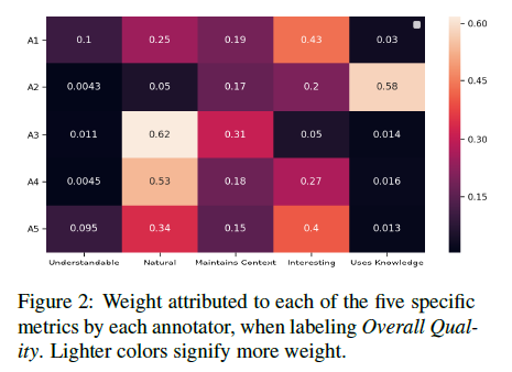
Mehri and Eskenazi (2020)[47] have shown that different dialog researchers weight quality aspects differently. Each researcher rates dialog responses for six quality aspects: Understandable, Natural (human-like), Maintains Context (coherent), Interesting, Uses Knowledge (factual consistent), and Overall Quality. A regression is then trained to map from the first five aspects to the Overall Quality. The ratings are normalized (using z-score) before training the regression. A softmax is computed over the regression weights. The Figure below shows the results from five annotators: A1 and A5 weight Interesting most; A2 weights Uses Knowledge most; and A3 and A4 weight Natural most.
Inter-Evaluator Agreement
In some open-domain chatbot papers, such as [4], [8], inter-evaluator agreement is reported for each quality aspect. A lower agreement indicates that the human evaluation metric is less reliable. Three different ways of measuring inter-evaluator agreement, Krippendorff’s \(\alpha\)[9],[10], Fleiss’ \(\kappa\)[51], and held-out correlation score[8], are discussed here.
Krippendorff’s \(\alpha\) is defined as \(\alpha=1-\frac{D_o}{D_e}\) where \(D_o\) and \(D_e\) are observed disagreement and expected disagreement by chance, respectively. For a set of generated responses \(X\) and a set of scores \(S\), let \(m,n\) denote index of \(S\) with values from 1 to \(\vert S\vert\), \(i\) denotes index of \(X\) with values from 1 to \(\vert X\vert\), and \((s_m,s_n)\) denotes score pairs assigned by evaluator pairs.
\[D_o=\sum\limits_{m=1}^{\vert S\vert}\sum\limits_{n=1}^{\vert S\vert} w_{m,n}\sum\limits_{i=1}^{\vert X\vert}\frac{\mathrm{number\ of\ evaluator\ pairs\ that\ assign\ x_i\ as\ }(s_m,s_n)}{\mathrm{total\ number\ of\ evaluator\ pairs}}\], where \(w_{m,n}\) is a weight for the \(m,n\) pair and a chosen distance measure between \(s_m\) and \(s_n\).
\[D_e=\sum\limits_{m=1}^{\vert S\vert}\sum\limits_{n=1}^{\vert S\vert} w_{m,n}r_{m,n}\], where \(r_{m,n}\) is the proportion of all evaluation pairs that assign scores \((s_m,s_n)\), which can be treated as the probability of two evaluators assigning scores \((s_m,s_n)\) to a generated response at random. Adiwardana et al. (2020)[4] showed that specificity metric has significantly lower Krippendorff’s \(\alpha\) than sensibleness metric and suggested that specificity is a more subjective metric than sensibleness.
Fleiss’ kappa. As opposed to Krippendorff’s \(\alpha\) that is based on the observed disagreement corrected for disagreement expected by chance, Fleiss’ \(\kappa\) is based on the observed agreement corrected for the agreement expected by chance. Fleiss’ \(\kappa\) is defined as \(\kappa=\frac{\bar P-\bar P_e}{1-\bar P_e}\), where \(1-\bar P_e\) is the degree of agreement attainable above chance, and \(\bar P-\bar P_e\) is the degree of agreement actually achieved above chance. Given \(N\) subjects, \(n\) ratings per subject, \(k\) categories of scale, \(i=1,...,N\) as index of subjects, and \(j=1,...,k\) as index of categories, \(n_{ij}\) is defined as the number of raters who assign the \(i\)-th subject to the \(j\)-th category and \(p_j=\frac{1}{Nn}\sum\limits_{i=1}^N n_{ij}\) is defined as the proportion of all assignments which are to the \(j\)-th category. Since \(\sum_j n_{ij}=n\), therefore \(\sum_j p_j=1\). The extent of agreement among the \(n\) raters for the \(i\)-th subject, \(P_i\), can be calculated by the proportion of agreeing pairs out of all the \(n(n-1)\) possible pairs of assignments: \(P_i=\frac{1}{n(n-1)}\sum\limits_{j=1}^k n_{ij}(n_{ij}-1)=\frac{1}{n(n-1)}(\sum\limits_{j=1}^k n_{ij}^2-n)\). The overall extent of agreement can be measured by the mean of the \(P_i\)s: \(\bar P=\frac{1}{N}\sum\limits_{i=1}^N P_i=\frac{1}{Nn(n-1)}(\sum\limits_{i=1}^N\sum\limits_{j=1}^k n_{ij}^2-Nn)\). If the raters make their assignments purely at random, the expected mean proportion of agreement is \(\bar P_e=\sum\limits_{j=1}^k p_j^2\).
Held-out correlation score is computed by holding out the ratings of one rater at a time, calculating its Pearson and Spearman correlations with the average of other rater’s judgments. The mean and max of all held-out correlation scores are reported as measures of inter-rater reliability. Pang et al. (2020)[8] compare the correlation between an automatic metric and a human evaluation metric to the inter-rater reliability of the human evaluation metric and consider the automatic metric to be reliable when the automatic-human correlation is close to inter-rater correlation.
Mehri and Eskenazi (2020)[40] introduced the FED (Fine-grained Evaluation of Dialog) dataset that contains 40 Human-Meena conversations, 44 Human-Mitsuku conversations, and 40 Human-Human conversations. Each conversation is annotated for 11 quality aspects at dialogue-level and three selected system responses per conversation are annotated for 9 quality aspects at turn-level, on 2-point or 3-point Likert scale answer options. Each data point is annotated by five annotators and the furthest label from the mean of the five is removed if its distance from the mean is greater than half the standard deviation of the five annotations. Inter-annotator agreement is computed by held-out Spearman correlation for each quality aspect. The agreement is high (0.68~0.84) for all the aspects, except “Understandable” (0.522) at turn-level and “Consistent” (0.562) at dialogue-level. At turn-level, Meena outperforms both Mitsuku and Human for all aspects, most noticeable for “Interesting”, “Engaging”, and “Specific”. At dialogue-level, Human outperforms both Meena and Mitsuku for all aspects. These results show that dialogue-level evaluation is more reliable than turn-level. To measure the contribution of each aspect to the overall impression, a regression is trained to predict the overall impression score given other quality aspects as input. A softmax is computed over the regression weights to determine the relative contribution of each quality aspect. The most important turn-level qualities are “Relevant” (18.10%), “Interesting” (16.15%), and “Fluent” (14.27%). The most important dialogue-level qualities are “Likable” (12.03%), “Understanding” (11.01%), and “Coherent” (10.95%).
Evaluator Bias Calibration
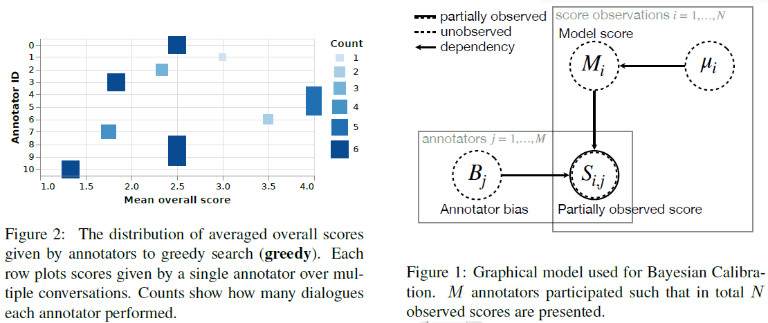
Kulikov et al. (2018)[13] interpret inter-evaluator variance as annotator bias, which comes from each annotator’s individual attitude towards and understanding of the task. To address this bias, they propose using Bayesian inference to account for the bias and the model’s underlying score, and report the posterior mean and variance of each model’s score as the calibrated score. The Bayesian inference is done in Pyro[14] using no-u-turn sampler[15]. Two types of evaluations, conversation-level Likert-type rating (4-point scale in their study, as shown in the left figure below) and utterance-level binary rating ({0, 1} for good or bad), are described.
For conversation-level Likert-type rating, both the unobserved score of the \(i\)-the model \(M_i\) and the unobserved bias of the \(j\)-th annotator \(B_j\) are treated as latent variables. The \(M_i\) is assumed to follow the normal distribution \(M_i\sim\mathcal{N}(\mu_i,1^2)\) and its mean is assumed to follow the uniform distribution \(\mu_i\sim\mathcal{U}(1,4)\). The \(B_j\) is assumed to follow the normal distribution \(B_j\sim\mathcal{N}(0,1^2)\). The observed score \(S_{ij}\) given by the \(j\)-th annotator to the \(i\)-the model is then \(S_{ij}\sim\mathcal{N}(M_i+B_j,1^2)\). The \(S_{ij}\) is a sampled subset of all observed scores \(\mathcal{O}\). The goal of inference is to infer the posterior mean \(\mathrm{\mathbb{E}}[M_i\vert\{S_{ij}\vert S_{ij}\in\mathcal{O}\}]\) and the variance \(\mathrm{\mathbb{V}}[M_i\vert\{S_{ij}\vert S_{ij}\in\mathcal{O}\}]\). The corresponding graphical model is shown in the right figure below.
For utterance-level binary rating, turn bias of \(k\)-th turn \(T_k\) is assumed to follow the normal distribution \(T_k\sim\mathcal{N}(0,1^2)\) and \(M_i\sim\mathcal{N}(0,1^2)\). The distribution of an observed score is assumed to follow Bernoulli distribution \(\mathcal{B}\): \(S_{ijk}\sim\mathcal{B}(\mathrm{sigmoid}(M_i+B_j+T_k))\). The goal of inference is to compute \(\mathrm{\mathbb{E}}_{M_i\vert\{S_{ijk}\vert S_{ijk}\in\mathcal{O}\}}[\mathrm{sigmoid}(M_i)]\) and \(\mathrm{\mathbb{V}}_{M_i\vert\{S_{ijk}\vert S_{ijk}\in\mathcal{O}\}}[\mathrm{sigmoid}(M_i)]\).
So far, few open-domain chatbot papers, such as [1], has applied Bayesian calibration on human evaluation scores.
Metrics Derived from Response Annotations
In some studies, quality metrics are derived from annotations, instead of just annotations themselves. Two examples are discussed here. Adiwardana et al. (2020)[4] defines Sensibleness and Specificity Average (SSA) as a simple average of Sensibleness and Specificity, which are percentage of responses annotated as sensible and specific, respectively. For sensible label, human annotator is asked to judge whether a response is completely reasonable in context. If a response is labeled as sensible, then the annotator is asked to judge whether it is specific to the given context. SSA is treated as a proxy for human likeness, because there is a high correlation between SSA and direct label of human likeness. Venkatesh et al. (2018)[16] evaluate coherence by response error rate (RER), defined as \(RER=\frac{Number\ of\ turns\ with\ erroneous\ responses}{Total\ number\ of\ turns}\), where erroneous responses include incorrect, irrelevant, or inappropriate responses as judged by human annotators.
Metrics Derived from User Behaviors
For chatbots deployed to live platform, such as in Amazon Alexa Prize competition[16], user usage behaviors, such as number of turns and duration of the conversation, have been used as a part of engagement metrics.
Reporting Standardization
The inconsistent usage of names and definitions of evaluated aspects across different papers and missing key details in reporting human evaluation experiments in some papers are common problems not only in open-domain chatbot studies but also in all other NLG studies over the last two decades[17]. To improve comparability, meta-evaluation, and reproducibility testing of human evaluations across NLG papers, Belz et al. (2020)[18] propose a classification system for human evaluation methods based on (i) what aspect of quality , named quality criterion, is being evaluated and (ii) how it is evaluated in specific evaluation modes and experimental designs. While they try to standardize a way of classifying evaluation methods, they do not propose a standardized nomenclature of quality criterion names and definitions. To further promote standardized reporting of human evaluation experiments in natural language processing (NLP), Shimorina and Belz (2021)[19] introduce the Human Evaluation Datasheet to be used as a template for recording the details of individual human evaluation experiments.
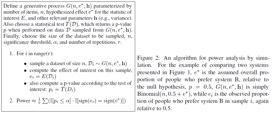
Another common problem in human evaluation studies in NLP is the ignorance of statistical power, resulting in underpowered performance comparisons in typical experimental design[20]. Statistical power is the probability that a statistical test will successfully detect a true effect, conditional on the experimental setting and significance threshold. When the power is less than 80%, it is considered as underpowered. Underpowered experiments may leave meaningful improvements to go undetected or apparently significant differences to be exaggerated. Card et al. (2020)[20] recommend that researchers should create an analysis plan and run power analyses, prior to evaluation experiment, to determine an appropriate sample size and improve the reliability and replicability of results. Their approach for power analysis is to estimate power by running simulations, using simulated datasets generated from assumed or estimated parameter values, as illustrated in the Figure below.
Automatic Evaluation
In addition to the lack of standardized definitions and reporting and the lack of power analysis, human evaluations incur cost to recruit crowdsourced evaluators, take longer to run, are not scalable to large number of models, and are not suitable for quick and frequent evaluations during system development. Thus, various forms of automatic evaluation metrics continue to be used for comparing open-domain chatbot models. Automatic metrics can be divided into two broad categories: traditional and machine-learning-based.
Traditional Automatic Metrics
Traditional automatic metrics, including n-gram-based, ranking-based, and linguistic-features-based, mostly compare single aspect of intrinsic qualities between generated responses and reference responses. They are used by a broad range of NLG tasks as common evaluation metrics. Although requiring a generated response to be highly similar to a small set of reference responses is reasonable to some NLG tasks, it may limit the diversity and interestingness of an open-domain chatbot. Some traditional automatic metrics have been shown to be poorly correlated with human evaluation metrics for dialogue systems[21].
N-Gram-Based Metrics
N-gram based metrics have been applied to measure lexical similarity between reference and generated responses, lexical diversity of generated responses, and factual consistency between generated response and grounding knowledge. When multiple values of the \(n\) in an n-gram-based metric are reported in the same paper, the notations of \(\mathrm{M}\! -\! n\) or \(\mathrm{M}_n\) for a given metric \(\mathrm{M}\) are used.
Lexical Similarity
Lexical similarity metrics measure n-gram overlap between generated and reference responses. Higher \(n\) of n-grams will capture more word order information, within n-grams, but will restrict the generated response to be more exactly matching the reference response. In most n-gram overlap methods, the order of n-grams is not considered, also known as bag of n-grams. Six lexical similarity metrics that are frequently encountered in open-domain chatbot papers are covered here: BLEU, NIST, F1-score, ROUGE, METEOR, and \(\Delta\)BLEU.
BLEU (Bilingual Evaluation Understudy), introduced by Papineni et al. (2002)[22], was originally developed for automatic evaluation of machine translation (MT). It is a weighted geometric mean of n-gram precision scores. It is usually calculated at the corpus-level, and was originally designed for use with multiple reference sentences. Applying it to a dialogue system, a response \(h\) is generated for a given conversation history \(c\) and an input message \(m\). A set of \(J\) reference responses \(\{r_{i,j}\}\) is available for the context \(c_i\) and message \(m_i\), where \(i\in\{1...I\}\) is an index over the test set. The BLEU-N score, where N is the maximum length of n-grams considered, of the system output \(h_1...h_I\) is defined as: BLEU-N \(=\) BP \(\cdot\exp\Big(\sum\limits_{n=1}^{\mathrm{N}}w_n\log\mathit{p}_n\Big)\) where brevity penalty (BP) is defined as BP=1 if \(\eta > \rho\) or BP=\(e^{(1-\rho/\eta)}\) if \(\eta\leq\rho\) where \(\eta\) and \(\rho\) are the lengths of generated and reference responses, respectively. The positive weights \(w_n=1/\mathrm{N}\) sum to one. The corpus-level n-gram precision \(p_n\) is defined as: \(p_n=\frac{\sum_i\sum_{g\in n-grams(h_i)}\mathrm{max}_j\{Count_g(h_i,r_{i,j})\}}{\sum_i\sum_{g\in n-grams(h_i)}Count_g(h_i)}\) where \(Count_g(\cdot)\) is the number of occurrences of an n-gram \(g\) in a given sentence, and \(Count_g(u,v)\) is a shorthand for \(\min\{Count_g(u),Count_g(v)\}\), the number of co-occurrences of the n-gram \(g\) in both \(u\) and \(v\). BLEU correlates strongly with human evaluation on MT task, but only weakly on non-MT tasks.
NIST, introduced by Doddington (2002)[24], is an improved version of BLEU for MT. First improvement is to use an arithmetic average of n-gram counts rather than a geometric mean, to reduce the potential of counterproductive variance due to low co-occurrences for the larger values of N. Second improvement is to weight more heavily those n-grams that occur less frequently, according to their information value. Thus, more informative n-grams contribute more to the score. Third improvement is a modification of brevity penalty to minimize the impact on the score of small variations in the length of a translation. Information weights are computed using n-gram counts over the set of reference translations/responses, according to the following equation: \(Info(w_1...w_n)=\log_2\Big(\frac{the\ \#\ of\ occurrence\ of\ w_1...w_{n-1}}{the\ \#\ of\ occurrence\ of\ w_1...w_n}\Big)\), where \(w\) denotes word/token and \(n\) is the length of the n-gram. When \(n=1\), the numerator is the total word/token count of the reference translations/responses set. The NIST score is
\[Score=\sum\limits_{n=1}^{N}\Bigg\{\frac{\sum\limits_{all\ w_1...w_n\ that\ co-occur}Info(w_1...w_n)}{\sum\limits_{all\ w_1...w_n\ in\ sysoutput}(1)}\Bigg\}\cdot\exp\Bigg\{\beta\log^2\Bigg[\min\Bigg(\frac{L_{sys}}{\bar{L}_{ref}},1\Bigg)\Bigg]\Bigg\}\]where \(N=5\), \(\beta\) is chosen to make the brevity penalty factor = 0.5 when the # of words in the system output is 2/3 of the average # of words in the reference translation, \(\bar{L}_{ref}=\)the average number of words in a reference translation, averaged over all reference translations, and \(L_{sys}=\)the number of words in the translation being scored. The NIST score provides significant improvement in score stability and reliability for all four translation corpora studied. For human evaluations of Adequacy, the NIST score correlates better than the BLEU score on all four translation corpora.
F1-score is the balanced harmonic mean of the precision (\(P\)) and recall (\(R\)), F1-score \(=\frac{2PR}{P+R}\). In standard F1-score[33], \(P\) and \(R\) are calculated using bag of n-grams approach. Let \(X\) and \(Y\) be the n-gram sets of reference and generated responses, respectively; then \(P=\frac{\vert X\cap Y\vert}{\vert Y\vert}\) and \(R=\frac{\vert X\cap Y\vert}{\vert X\vert}\). To take n-gram order into consideration, Melamed et al. (2003)[23] introduced GTM (General Text Matcher) score that uses bitext grid to define maximum matching size (MMS) between reference and generated responses, in which double-counting is avoided and contiguous sequences of matching words are rewarded in proportion to the area of non-conflicting aligned blocks. Let \(V\) and \(W\) be the texts of reference and generated responses, respectively, then GTM score is computed by the F1-score using \(P=\frac{MMS(W,V)}{\vert W\vert}\) and \(R=\frac{MMS(W,V)}{\vert V\vert}\). GTM score significantly outperforms BLEU on evaluating MT, especially on shorter document and fewer references, as judged by their correlations with human evaluation of Adequacy. However, F1-score can be gamed by exploiting common n-grams. To rectify this, Shuster et al. (2021)[7] introduced Rare F1 (RF1) metric that only considers infrequent words in the dataset when calculating F1-score. An infrequent word is defined as a word in the lower half of the cumulative frequency distribution of the reference corpus. RF1 score correlates better than standard F1-score with human evaluation scores of consistency, engaging, knowledge, and hallucinate.
ROUGE (Recall-Oriented Understudy for Gisting Evaluation), introduced by Lin (2004)[25], is a set of metrics for automatic evaluation of computer-generated summaries in comparison with ideal summaries created by humans. ROUGE-N is an n-gram recall between a candidate summary and a set of reference summaries. ROUGE-N = \(\frac{\sum\limits_{S\in\{ReferenceSummaries\}}\sum\limits_{gram_n\in S}Count_{match}(gram_n)}{\sum\limits_{S\in\{ReferenceSummaries\}}\sum\limits_{gram_n\in S}Count(gram_n)}\), where \(gram_n\) denotes an n-gram of length \(n\) and \(Count_{match}(gram_n)\) is the maximum number of n-grams co-occurring in a candidate summary and a set of reference summaries. To compute ROUGE-N between a candidate summary \(s\) and multiple references, pairwise score between \(s\) and every reference \(r_i\) in the reference set is computed first. Then, the maximum of pairwise scores is used as the final score: \(\mathrm{ROUGE\! -\! N_{multi}}=\mathrm{argmax}_i\mathrm{ROUGE\! -\! N}(r_i,s)\). Instead of just getting a single score from M references, an average of M scores can be obtained by a Jackknifing procedure: first computing the best score over M sets of M-1 references, then taking an average of the M scores. Contrary to the bag of n-grams approach of ROUGE-N, ROUGE-L uses longest common subsequence (LCS) to measure similarity between reference and candidate sentences. LCS requires multiple n-grams to be in order, but not consecutive. ROUGE-L is defined as LCS-based F-measure: given \(X\) of length \(m\) and \(Y\) of length \(n\) as a reference sentence and a candidate sentence, respectively, LCS-based recall is \(R_{lcs}=\frac{LCS(X,Y)}{m}\), LCS-based precision is \(P_{lcs}=\frac{LCS(X,Y)}{n}\), and ROUGE-L is \(F_{lcs}=\frac{(1+\beta^2)R_{lcs}P_{lcs}}{R_{lcs}+\beta^2P_{lcs}}\), where \(LCS(X,Y)\) is the length of a longest common subsequence of \(X\) and \(Y\), and \(\beta=P_{lcs}/R_{lcs}\) controls the relative importance of \(P_{lcs}\) and \(R_{lcs}\). When applying to multi-sentence summary-level for a reference summary of \(u\) sentences containing a total of \(m\) words and a candidate summary of \(v\) sentences containing a total of \(n\) words, the summary-level LCS-based F-measure can be computed as follows: \(R_{lcs}=\frac{\sum\limits_{i=1}^u LCS_{\cup}(r_i,C)}{m}\), \(P_{lcs}=\frac{\sum\limits_{i=1}^u LCS_{\cup}(r_i,C)}{n}\), and \(F_{lcs}=\frac{(1+\beta^2)R_{lcs}P_{lcs}}{R_{lcs}+\beta^2P_{lcs}}\), where \(LCS_{\cup}(r_i,C)\) is the LCS score of the union of all the LCS between \(r_i\) and each sentence of a candidate summary \(C\). ROUGE-S, based on skip-bigram co-occurrence statistics, and several other ROUGE variants are less frequently used and not discussed here. Different ROUGE variants perform better at different experimental settings on evaluating document summarization tasks, as judged by correlations with human evaluations.
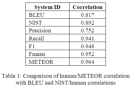
METEOR (Metric for Evaluation of Translation with Explicit ORdering), introduced by Banerjee and Lavie (2005)[26], is designed to explicitly address four weaknesses of BLEU: (1) the fixed brevity penalty in BLEU does not adequately compensate for not using recall; (2) BLEU does not explicitly measure word order (related to grammaticality), but uses higher order n-grams to indirectly measure word order; (3) BLEU’s bag of n-grams approach may result in counting incorrect word matches; (4) BLEU is intended to be used only for aggregate counts over an entire test-set and can be meaningless at the sentence level. METEOR creates an alignment between a system translation and a reference translation, where an alignment is defined as a mapping between unigrams, such that every unigram in each string maps to zero or one unigram in the other string, and to no unigrams in the same string. This alignment is incrementally produced through a series of stages, each by a different external module, such as exact module, porter stem module, and WN synonymy module. Each stage consists of two distinct phases: (1) an external module lists all the possible unigram mappings between the two strings, and (2) the largest subset of these unigram mappings is selected as the alignment. When multiple subsets are the largest, the one with the least number of unigram mapping crosses is selected as the alignment. Each stage only maps unigrams that have not been mapped to any unigram in any of the preceding stages; thus, the order of applying the external modules matters. By default, the order is exact module > porter stem module > WN synonymy module. Once all the stages have been run and a final alignment has been produced, the alignment can be used to find the \(\#unigram\_matched\) that is the number of unigrams in the system translation that are mapped and the \(\#chunks\) that is the minimal number of groups of mapped unigrams in adjacent positions. Then unigram precision \(P\) and unigram recall \(R\) are calculated as \(P=\frac{\#unigram\_matched}{\#unigrams_{sys}}\) and \(R=\frac{\#unigram\_matched}{\#unigrams_{ref}}\). Finally, the METEOR score is defined as \(Score=Fmean\times(1-Penalty)\), where \(Fmean\) is a harmonic mean of 1 \(P\) and 9 \(R\), \(Fmean=\frac{10PR}{R+9P}\) and \(Penalty=0.5\times(\frac{\# chunks}{\# unigram\_matched})^3\). In case of multiple references for a system translation, the best score is used. System level METEOR score is calculated by micro-averaging the \(P\), \(R\), and \(Penalty\) over the entire test set, and then combining them using the same formula as the sentence level METEOR score. The Table below shows the system level correlation between human judgments and various MT evaluation metrics and sub components of METEOR.
However, on evaluating dialogue systems, BLEU-N, ROUGE, and METEOR have been shown to correlate poorly with human judgements[21].
\(\Delta\)BLEU (Discriminative BLEU), introduced by Galley et al. (2015)[27], is designed to improve BLEU for evaluating tasks that allow a diverse range of possible outputs. The idea is to first create a test set of conversational data that contains 16 diverse reference responses for each context and input message. Then, a weight is assigned by human annotators to each reference response. Finally, the human-assigned weight of each reference response is included in computing the corpus-level n-gram precision \(p_n\) of the BLEU score. Using the same notations as those in the BLEU section above, the \(p_n\) of the \(\Delta\)BLEU is defined as: \(p_n=\frac{\sum_i\sum_{g\in n-grams(h_i)}\mathrm{max}_{j:g\in r_{i,j}}\{w_{i,j}\cdot Count_g(h_i,r_{i,j})\}}{\sum_i\sum_{g\in n-grams(h_i)}\mathrm{max}_j\{w_{i,j}\cdot Count_g(h_i)\}}\), where \(w_{i,j}\in[-1,+1]\) is the human assigned weight associated with the reference \(r_{i,j}\). To ensure that the denominator is never zero, it is assumed that, for each \(i\) there exists at least one reference \(r_{i,j}\) whose weight \(w_{i,j}\) is strictly positive. Higher-valued positive-weighted references are typically reasonably appropriate and relevant; negative-weighted references are semantically orthogonal to the intent of their associated context and message. The quality of the \(\Delta\)BLEU-2 and BLEU-2 are evaluated by their rank correlations (Spearman’s \(\rho\) and Kendall’s \(\tau\)) with human evaluation on relevance to both context and message. \(\Delta\)BLEU achieves better correlation with human evaluation than BLEU, although the correlations are still weak (\(\rho=0.484, \tau=0.342\) for \(\Delta\)BLEU and \(\rho=0.318, \tau=0.212\) for BLEU).
Although the lexical similarity metrics discussed above are developed for comparing generated and reference texts, they have been applied similarly to measure coherence or n-gram reuse between generated responses and dialogue context. Berlot-Attwell and Rudzicz (2021)[36] calculated n-gram precision between the stemmed response and the stemmed context for 2-, 3-, and 4-grams as a metric of n-gram reuse. Stemming is performed using NLTK. Unlike BLEU, there is no brevity penalty or average over n from 1 to N.
Lexical Diversity
Lexical richness or diversity of generated text is a desired quality in some NLG tasks, including open-domain chatbots[8]. The commonly used n-gram-based metrics for evaluating lexical diversity are covered here, including TTR, distinct-n, LS2, unique-n, Shannon text entropy, conditional next-word entropy, and Self-BLEU.
TTR (Type-Token Ratio)[28] defines “type” as distinct word/token and \(TTR=\frac{Count(distinct\ tokens)}{Count(total\ tokens)}\) of all the generated responses for the test set. However, TTR is sensitive to sample size and tends to decrease as the sample size increases. One way to address the issue is MSTTR (Mean Segmental TTR), which divides the generated responses into successive segments of a given length (e.g. 50 tokens) and then calculates the mean of all segmental TTRs.
Distinct-n is defined as \(\mathrm{distinct}\! -\! n=\frac{Count(distinct\ n-grams)}{Count(total\ n-grams)}\), which can be applied at conversation level[13] or corpus level. When applied at conversation level, the metric is computed for each generated conversation turn and then averaged over the test set. When applied at corpus level for unigrams, it is identical to TTR.
Lexical sophistication (LS2)[13], also known as lexical rareness, measures the proportion of relatively unusual or advanced words in the generated text: \(LS2=\frac{Count(distinct\ rare\ words)}{Count(distinct\ words)}\) of all generated responses on the test set, where rare words can be the word types not on the list of 2000 most frequent words generated from the British National Corpus. Unique-n[29] is another way to measure relatively rare word usage: the count of n-grams that only appear once across the entire test output.
Shannon text entropy quantifies the amount of variation in generated texts. Texts with higher lexical diversity will have higher entropy. The entropy \(H\) of all generated responses \(G\) is defined[28] as \(H(G)=-\sum\limits_{x\in S_n}\frac{freq(x)}{total}\times \log_2(\frac{freq(x)}{total})\), where \(x\) denotes an unique n-gram, \(S_n\) denotes the set of all unique n-grams in \(G\), \(freq(x)\) denotes the number of occurrences of \(x\) in \(G\), and \(total\) denotes total number of n-grams in \(G\). \(H_1\), \(H_2\), and \(H_3\) represent entropies of unigrams, bigrams, and trigrams, respectively. Conditional next-word entropy measures the diversity of the next word given one (bigram) or two (trigram) previous words: \(H_{cond}(G)=-\sum\limits_{(c,w)\in S_n}\frac{freq(c,w)}{total}\times \log_2(\frac{freq(c,w)}{freq(c)})\), where \((c,w)\) denotes an unique n-gram composed of \(c\) (context, all tokens but the last one) and \(w\) (the last token). The more diverse a text is, the less predictable is the next word given previous word(s) and, thus, the higher is the conditional next-word entropy.
Self-BLEU has been proposed by Zhu et al. (2018)[30] as a metric to evaluate the diversity of generated responses. Regarding one generated response as hypothesis and the others generated responses as references, a BLEU score is calculated for every generated response, and the average BLEU score is defined as the Self-BLEU of the test set. A higher Self-BLEU score implies less diversity among the generated responses.
Factual Consistency
In knowledge-grounded dialogue system, generated responses are expected to be factually consistent with its corresponding ground-truth knowledge. N-grams-based metrics for evaluating factuality of generated responses are covered here, including Knowledge F1 and Wiki F1.
Knowledge F1 (KF1), introduced by Shuster et al. (2021)[7], measures unigram overlap F1-score between generated response and ground-truth knowledge as judged by humans during test dataset collection. This metric is designed to evaluate retrieval-augmented dialogue models using test datasets that provide gold knowledge at every turn, such as Wizard of Wikipedia (WoW) and CMU Document Grounded Conversations (CMU_DoG). KF1 score has very strong correlation with human evaluation scores of Knowledge (Pearson’s \(r=0.94\)) and Hallucinate (Pearson’s \(r=-0.95\)). A similar metric called Wiki F1 score has been introduced by Dinan et al. (2018)[31] to assess how knowledgeable a chatbot is.
Ranking-Based Metrics
There are three types of architectures in building open-domain chatbots: retrieval-based, generation-based, and hybrid. Ranking-based metrics are only used for evaluating retrieval-based chatbots, which retrieve candidate responses from a pre-collected human conversational dataset according to some matching scores between an input context and the candidate responses. In the datasets, multiple context-response pairs have the same context but different responses, each with a positive/negative labels. Different datasets may have different positive:negative ratio, typically from 1:1 to 1:9. Commonly used ranking-based metrics[32] for evaluating retrieval-based open-domain chatbots are covered here, including \(\mathrm{R}_n@k\), \(\mathrm{P}@k\), \(\mathrm{Hits}@1/N\), MRR, and MAP.
\(\mathrm{R}_n@k\) is recall at \(k\) from \(n\), meaning the recall of the true positive responses among the \(k\) best-matched responses from \(n\) available candidates for the given conversation context. \(\mathrm{R}_n@k=\frac{\sum_{i=1}^k y_i}{\sum_{i=1}^n y_i}\), where \(y_i\) is the binary label for each candidate.
\(\mathrm{P}@k\) is precision at \(k\), meaning the number of positive responses in the top \(k\) selections divided by \(k\) for each test instance. Then, average \(\mathrm{P}@k\) is the macro-average of \(\mathrm{P}@k\) over the test set. In case of \(k=1\), the per-instance score is either 1 or 0; thus, the average \(\mathrm{P}@1\) is the number of test instances whose 1st-ranked response is positive divided by the total number of test instances.
\(\mathrm{Hits}@1/N\)[33] is the accuracy of the generated response when choosing between the gold response and \(N-1\) distractor responses.
MRR (mean reciprocal rank) score is defined as the average of reciprocal rank over the whole testing set, where the reciprocal rank of a test instance is defined as the reciprocal of the rank of the first positive response. \(\mathrm{MRR}=\frac{1}{\vert T\vert}\sum\limits_{i=1}^{\vert T\vert}\frac{1}{rank_i}\), where \(\vert T\vert\) is the number of test instances and \(rank_i\) is the rank position of the first positive response for the i-th test instance.
MAP (mean average precision) score is defined as the mean of average precision (AP) over the whole test set. The AP for each test instance is defined as \(\mathrm{AP}=\frac{\sum_{k=1}^n\mathrm{P}@k\ \times Ind(k)}{Count(positive\ responses)}\) in \(n\) top-matched responses, where \(Ind(k)\) is 1 or 0 corresponding to the positive or negative label, respectively, and \(Count(positive\ responses)\) is the number of positive responses in the \(n\) top-matched responses of the test instance. \(\mathrm{MAP}=\frac{1}{\vert T\vert}\sum\limits_{i=1}^{\vert T\vert}\mathrm{AP}_i\)
Perplexity
Word perplexity is a well-established metric for comparing probabilistic language models (LMs), ranging from classical n-gram LMs to modern transformer-based LMs. Word perplexity has also been widely used for evaluating generation-based[34] and hybrid[7] open-domain chatbots. For a test dialogue dataset containing \(N\) instances of context \(c\) and reference response \(r\), word perplexity is defined as \(\exp\Big(-\frac{1}{N_W}\sum\limits_{n=1}^N\sum\limits_{t=1}^{T_r}\log P_{\theta}(r_{n,t}\vert r_{n,<t}, c_n)\Big)\), where \(N_W\) is the total number of tokens in all the reference responses, \(T_r\) is the total number of tokens in the reference response \(r\), and \(\theta\) is model parameters. Perplexity explicitly measures the model’s ability to account for the syntactic structure of the dialogue and the syntactic structure of each utterance. Perplexity metric always measures the probability of regenerating the exact reference utterance. Lower perplexity is indicative of a better model. Perplexity is not comparable between models with different vocabularies or trained from different corpora. Pang et al. (2020)[8] define response fluency score as negative perplexity of generated responses and show that the generated response fluency metric (normalized to be in the range [0,1]) is highly correlated with human judgement.
Linguistic-Knowledge-Based Metrics
Linguistic knowledge, such as synonyms, lemmas, contentful words, and grammaticality, have been used to measure similarity between generated responses and reference responses or context, or to measure intrinsic quality of generated responses.
SynSet Distance between a generated response and a reference response, introduced by Conley et al. (2021)[35], is defined as \(\frac{\vert S_g\ \cap\ S_r\vert}{\vert S_g\ \cup\ S_r\vert}\), where \(S_g\) and \(S_r\) denote the set of synonyms and lemmas retrieved from WordNet by the words of generated response and reference response, respectively. The ratio of the size of the intersection set to the size of the union set of the two sets provides a distance measurement between 0 (no similarity) and 1 (identical).
Acknowledgement is defined by Berlot-Attwell and Rudzicz (2021)[36] as percentage of contentful words in the response having a synonym within the context. The contentful words of the response are nouns, verbs, adverbs, and adjectives that are not stop words, extracted using spaCy. Synonyms are determined using WordNet. If the response contains no contentful parts of speech, then NaN is returned.
Grammaticality is defined by Berlot-Attwell and Rudzicz (2021)[36] as \(1-\frac{\#errors}{\#tokens}\), where \(\#errors\) denotes the number of Grammar, Collocation, and Capitalization errors detected by rule-based LanguageTool in the response and \(\#tokens\) denotes the response length.
Machine-Learning-Based Automatic Metrics
Machine-learning-based automatic metrics can be divided into three categories: aspect-specific-classifier-based, word-embedding-based, and learning-based. An aspect-specific classifier approach trains a classifier to evaluate a single aspect of a text or a relation of texts, which is then used to formulate a dialog quality metric. A word embedding approach directly uses pre-trained word embeddings to represent contexts and responses of dialogs and uses embedding distances to formulate a dialog quality metric. A learning-based approach trains a model specifically for dialog quality scoring task.
Aspect-Specific-Classifier-Based Metrics
Fine-grained aspects of conversation qualities can often be evaluated using specialized classifiers that provide labels for utterances or context. The probabilities or counts of the labels can then be used for computing final metrics scores. In some case, class labels are directly assigned with some numerical values that are then used to compute metric scores. Most of these metrics do not require gold-label reference responses. Six examples are covered here: Topic Depth and Breadth, Predictive Engagement, Logical Self-Consistency, Sentiment Distance, Acceptability, and \(Q^2\) for Factual Consistency.
Topic Depth and Breadth. Amazon Alexa Prize competition uses an Attentional Deep Average Network (ADAN) model[37] to classify the topic and the topic-wise word saliency for each input utterance. A series of topic related metrics are defined for the evaluation of open-domain chatbots. Topic-specific turn \(\mathcal{T}\) is a pair of user utterance and bot response where both belong to the same topic, excluding Phatic that does not have a defined topic. Topic coherent sub-conversation \(\mathcal{S}\) is a series of two or more consecutive topic-specific turns of the same topic, and the Phatic turn is excluded. Length of sub-conversation \(l_s\) is the number of turns a topic coherent sub-conversation contains. Length of consecutive conversation \(l_c\) is the total number of consecutive topic-specific turns, whose topics do not need to be the same. For a conversation \(C_i\) with \(m\) sub-conversations \(S_{ij}\) where \(j=1,...,m\), dialog-level average topic depth \(D(C_i)\) is the average length of all sub-conversations in each user-bot conversation: \(D(C_i)=\frac{1}{m}\sum_{j=1}^m l_s(S_{ij})\) and system-level average topic depth \(D(\mathcal{B})\) is the average length of all sub-conversations \(C_i\), \(i=1,...,n\) generated by a chatbot \(\mathcal{B}\). Dialog-level coarse topic breadth \(Br(C_i)\) is the number of distinct topics \(t_k\) that occur during at least one sub-conversation in conversation \(C_i\). System-level coarse topic breadth \(Br_{avg}(\mathcal{B})=\frac{1}{n}\sum_{i=1}^n Br(C_i)\), where \(n\) is the number of conversations generated by bot \(\mathcal{B}\). System-level coarse topic count \(N(\mathcal{B},t_k)\) is the total number of sub-conversations with topic \(t_k\) in all conversations \(C_i\) by \(\mathcal{B}\). The histogram of \(N(\mathcal{B},t_k)\) across topics shows whether a bot mostly talks about a few topics or tends to talk equally about a range of topics. Normalizing the histogram result in the System-level coarse topic frequency \(F(\mathcal{B}, t_k)\). The top-2 most salient keywords per utterance detected by ADAN are used to compute topic keyword related metrics. System-level topic keyword coverage \(C_{fine}(\mathcal{B})\) is the total number of distinct topic keywords across all conversations \(C_i\) generated by conversational bot \(\mathcal{B}\). System-level topic keyword count \(N(\mathcal{B}, w_k)\) is the total count of topic keywords \(w_k\) across all conversations \(C_i\) by \(\mathcal{B}\). Averaging over topic keywords results in the System-level topic keyword frequency \(F(\mathcal{B}, w_k)\). The results show that the topic depth \(D(\mathcal{B})\) correlates better with the human judgment (on liking to speak again) than the conversation length (regardless of topics), indicating that the user is more satisfied if the bot is able to sustain longer sub-conversations on the same topic. The average topic breadth \(Br_{avg}(\mathcal{B})\) within each conversation correlates reasonably well with user ratings, which means that when users chat with a bot about various topics in the same conversation, they tend to rate the bot higher.
Predictive Engagement. Ghazarian et al. (2019)[52] introduced a predictive engagement metric that provides utterance-level engagement measurement and improves correlation to human judgements of dialog utterances when combined with a relevance metric. Here, engagement is defined as a user’s inclination to continue interacting with a dialogue system. All earlier human evaluations of dialog engagement were at conversation-level. ConvAI dataset includes human annotated conversation-level engagement scores in the range of 0 to 5, corresponding to not engaging at all to extremely engaging. In order to use this dataset for training a binary classifier at utterance-level, all utterances of a conversation are assigned the same engagement score as the conversation and the scores 0~2 and scores 3~5 are grouped into not engaging and engaging, respectively.
To justify the assignment of utterance-level engagement scores directly by using their corresponding conversation-level engagement scores, two sets of correlation studies were conducted. First, aggregated (mean) human-annotated utterance-level engagement scores show high Pearson correlation (0.85) with conversation-level engagement scores. Second, human-annotated utterance-level engagement scores show a relatively high Pearson correlation (0.60) with utterance-level engagement scores inherited from conversation-level engagement scores.
The binary engagement classifier (EC) is illustrated in the Figure below. The utterance vectors are computed by simply taking the max or mean pooling of their contextualized word embeddings encoded by BERT. The utterance vectors of query and response pairs are then averaged and used as input to a Multilayer Perceptron (MLP) classifier that uses cross-entropy loss to classify the utterance as 0 (not engaging) or 1 (engaging). After the training with the ConvAI dataset, the utterance-level EC is fine-tuned with a small set of utterances pairs randomly selected from the Daily Dialog dataset. The fine-tuning utterances pairs have been annotated as engaging or not engaging, with mean \(\kappa\) agreement of 0.51 between annotators.
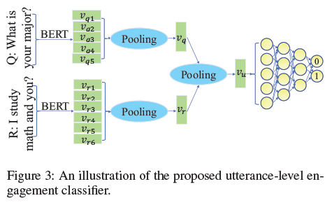
To evaluate the EC, with mean or max pooling, the unreferenced score (measuring relevance) of RUBER and BERT-RUBER are used as the baseline metrics. The evaluation dataset includes 300 utterances with generated replies and 300 utterances with human-written replies from the same 300 queries randomly selected from the Daily Dialog dataset. The correlation between human evaluation score of overall quality and one of the following 6 metrics are compared: RUBER_relevance, BERT_RUBER_relevance, EC_mean, EC_max, avg of (EC_mean, BERT_RUBER_relevance), and avg of (EC_max, BERT_RUBER_relevance). The results show that the incorporation of engagement scores into relevance scores yields scores significantly closer to human judgements than either engagement scores or relevance scores alone.
Logical Self-Consistency. Pang et al. (2020)[8] use a pre-trained Multi-Genre Natural Language Inference (MNLI) model to label if the relation of the response and the utterance history of the same agent is logically consistent. The model is a ternary classifier that takes two utterances as input and predicts the relation as either contradiction, entailment or neutral on the MNLI dataset. The contradiction score is defined as the average of the contradiction class probabilities of the current utterance and each prior utterance from the agent. The final score of logical self-consistency is defined as \(1-\mathrm{contradiction\ score}\). To increase the chance of producing self-contradictory responses, the queries are paraphrased by (1) replacing some words with synonym defined in WordNet, or (2) generating a different query with Conditional Text Generator (CTG) model conditional on the context. The results show that the metric based on paraphrasing augmented data has much stronger correlation with human evaluation than that not based on augmented data. In particular, the metric based on CTG augmentation correlates (Pearson’s \(r=0.65\), Spearman’s \(\rho=0.66\)) better than that based on WordNet Substitution.
Sentiment Distance. Conley et al. (2021)[35] use a Naive Bayes Analyzer to provide a simple measure of positive or negative sentiment for each utterance. A simple difference of the positive probabilities between a generated response and a reference response is defined as Sentiment Distance, with values between 0 and 1.
Acceptability. Berlot-Attwell and Rudzicz (2021)[36] use a biLSTM-based sentence encoder and a lightweight binary classifier to label utterances as acceptable or unacceptable, pre-trained on the Corpus of Linguistic Acceptability (CoLA). The acceptability covers morphological, syntactic, and semantic correctness. The metric, the probability of acceptable label, has similarly high scores across several different generative architectures for chatbots.
\(Q^2\) for Factual Consistency. Honovich et al. (2021)[46] introduced \(Q^2\) metric for evaluating factual consistency of generative open-domain knowledge-grounded dialog systems, which compares answer spans using a natural language inference (NLI) model. In knowledge-grounded dialog systems, each response is expected to be consistent with a piece of external knowledge, such as a Wikipedia page, a Washington Post article, or some fun-facts from Reddit, depending on the grounding dataset. Instead of directly measuring consistency between a response and its corresponding grounding knowledge, \(Q^2\) focuses on key information in the response and uses them as “answers” to generate questions that in turn are used to generate answers with the grounding knowledge. The response-extracted answer and the corresponding knowledge-grounded answer are then used to generate a consistency score. The \(Q^2\) pipeline consists of four steps. (1) All named entities and noun phrases in a response \(r\) are marked by spaCy as informative spans \(a_i^r\). (2) For each informative span \(a_i^r\), \(Q^2\) uses a question generation (QG) model, T5-base fine-tuned on SQuAD1.1, to generate questions \(q_{i_j}\) whose answer is \(a_i^r\). The QG model can be denoted as \((q_{i_j}\vert r,a_i^r)\). The decoding process of the QG model uses beam search with width of 5. The 5 generated questions are checked by the validation filtering (described below) and invalid questions are discarded. (3) For each question \(q_{i_j}\), \(Q^2\) uses an extractive question answering (QA) model, Albert-Xlarge model fine-tuned on SQuAD2.0, to mark an answer span \(a_{i_j}^k\) from grounding knowledge \(k\). The QA model can be denoted as \((a_{i_j}^k\vert k,q_{i_j})\). In the validation filtering step, a \(q_{i_j}\) is designated as invalid, if the \(a_{i_j}^r\) from \((a_{i_j}^r\vert r,q_{i_j})\) is not identical to \(a_i^r\). (4) \(Q^2\) then measures the similarity of \(a_i^r\) and \(a_{i_j}^k\) and aggregates the similarity scores for all questions as the factual consistency score of \(r\).
For answer span pairs \(a_i^r\) and \(a_{i_j}^k\) that match perfectly at the token-level, a score of 1 is assigned; otherwise, an NLI model, RoBERTa fine-tuned on Stanford NLI corpus, is run by using \(q_{i_j}+a_{i_j}^k\) as the premise and \(q_{i_j}+a_i^r\) as the hypothesis, where \(+\) denotes string concatenation. The \(q_{i_j}\)’s score is set to \(1\) for entailment case and \(0\) for contradiction case or for cases where the QA model produced no answer. For neutral case, the token-level F1 between the answer span pair is used as the score. Finally, the pair-level match scores for all pairs of a response are averaged to yield a response-level score, and the response-level scores are averaged to yield a system-level score. For the responses that do not have any valid generated question, the NLI model is used with \(r\) as the premise and \(k\) as the hypothesis. The score is set to \(1\) for entailment, \(0\) for contradiction, and \(0.5\) for neutral.
To evaluate \(Q^2\), a dataset of knowledge-grounded dialogue responses and their annotated factual consistency with respect to a given knowledge is created. A random sample of responses from two dialog systems, MemNet and dodecaDialogue, on the Wizard of Wikipedia (WoW) validation set are annotated by three annotators for factual consistency. The resulting dataset contains 544 dialog contexts and 1,088 annotated responses. Out of the 544 contexts, 186 (34.2%) were marked as inconsistent in the dodecaDialogue system and 274 (50.36%) in the MemNet system. The quality of the constructed dataset is shown by high inter-annotator agreement, Fleiss’ kappa = 0.853. \(Q^2\) score is indeed always highest (0.696 for dodeca, 0.756 for MemNet) for the consistent outputs, lowest (0.238 for dodeca, 0.135 for MemNet) for the inconsistent outputs, and in-between (0.496 for dodeca, 0.448 for MemNet) for random samples. Dropping the NLI component and using the fallback token-level F1 instead, result in lower \(Q^2\) score for both consistent and inconsistent responses, and by a larger margin for the former. The scores for the consistent data are also higher than the scores for the inconsistent data for all the four baseline metrics: BLEU, BERTScore, F1 token-level overlap of \(r\) with \(k\), and end-to-end NLI taking \(k\) as the premise and \(r\) as the hypothesis. However, in most cases, the score differences between the inconsistent data and the random samples are small, indicating that \(Q^2\) better separates general responses from inconsistent ones. The Spearman correlation of system-level \(Q^2\) and the four baseline metrics with the human judgment scores show that \(Q^2\) obtains an average correlation of 0.9798, while the end-to-end NLI baseline, overlap, BERTScore, and BLEU obtain lower correlations of 0.9216, 0.878, 0.8467 and 0.3051, respectively. To evaluate \(Q^2\)’s ability in automatically separating between consistent and inconsistent responses at single response level, the Precision-Recall curves of consistent responses is calculated for various response-level score thresholds for each evaluated metric on the WoW annotated data. The results show that \(Q^2\) obtains higher precision and recall in comparison to the four baseline metrics throughout the threshold values, suggesting that \(Q^2\) is better at automatically separating between consistent and inconsistent examples at the response level.
Embedding-Based Metrics
Word embeddings are dense vectors for words, which can be encoded by neural autoencoders, derived from matrix factorization of word-word co-occurrence matrix, or encoded by transformer-based language models. Word embeddings capture fine-grained semantic and syntactic regularities using vector arithmetic and thus can be used directly to measure distance in vector space. Static word embedding of a word is fixed regardless of surrounding words and does not capture word order or compositionality. Contextual word embedding captures different vector representations for the same word in different sentences depending on the surrounding words, and potentially captures sequence information.
There are three common approaches to measure similarity between two sentences using their constituent word embeddings, without additional learning. (1) Greedy Matching. Each word in the generated sentence is greedily matched to a word in the reference sentence based on the cosine similarity of their embeddings. The final score is then an average of all word scores of the generated sentence. (2) Vector Extrema computes a sentence embedding by taking the maximum value of each dimension of the embeddings of all the words of the sentence. The final score is then the cosine similarity between sentence embeddings. (3) Embedding Average computes a sentence embedding by taking an average of word embeddings. The final score is then the cosine similarity between sentence embeddings. In some studies[47], Vector Extrema has been shown to perform better than the other two approaches on dialog tasks; but in others[48], each of the three approaches may perform better than the other two, dependent upon the chatbot model and test dataset.
Conley et al. (2021)[35] define Embedding Distance between a generated response and a reference response as \(\frac{\vert S_g^{\prime}\ \cap\ S_r^{\prime}\vert}{\vert S_g^{\prime}\ \cup\ S_r^{\prime}\vert}\), where \(S_g^{\prime}\) and \(S_r^{\prime}\) denote the set of the n-closest words (in terms of Euclidean distance of pretrained GloVe word embeddings) from each word in generated response and reference response, respectively. The value of the ratio is between 0 and 1. They also define Cosine Distance between a generated response and a reference response as the cosine distance between the average word embeddings of the words of each response. Cosine similarity, \(cos(\theta)=\frac{\vec A\cdot\vec B}{\Vert\vec A\Vert\ \Vert\vec B\Vert}\), of two real-valued vectors, \(\vec A\) and \(\vec B\), has values in range [-1, 1]. Cosine distance, typically defined as 1 - cosine similarity, will have values in range [0, 2].
Berlot-Attwell and Rudzicz (2021)[36] define Semantic Relatedness between a generated response and its context as the average cosine distance between the contentful words in generated response that do not have a synonym in the context. The word embedding are obtained from GloVe vectors pre-trained on the Twitter Corpus. The cosine distance for such a contentful word is determined between the contentful word and the most similar word in the context. Words without a corresponding GloVe vector are ignored. The Semantic Relatedness is defined to be 0 if there are no contentful words without a synonym in the context. Unfortunately, this metric did not perform well as shown in the results that the distribution of relatedness of the gold response is very similar to that of the Random baseline.
BERTScore. Zhang et al. (2019)[38] introduce BERTScore based on pre-trained BERT contextual embeddings to evaluate semantic equivalence. BERTScore computes the similarity of two sentences as a sum of cosine similarities between their tokens’ embeddings. BERT tokenizes the input text into a sequence of word pieces, where unknown words are split into several commonly observed sequences of characters. Given a tokenized reference sentence \(x=\langle x_1,...,x_k\rangle\) and a tokenized candidate sentence \(\hat x=\langle \hat x_1,...,\hat x_m\rangle\), the embedding model generates a sequence of vectors \(\langle\mathrm{x}_1,...,\mathrm{x}_k\rangle\) and \(\langle\mathrm{\hat x}_1,...,\mathrm{\hat x}_m\rangle\), respectively. The best layer in a transformer-based model to obtain contextual embeddings for BERTScore varies by the specific model used. For example, the 9th and 18th layers are the best from the 12-layered BERT-base and 24-layered BERT-large, respectively. The vectors \(\mathrm{x}_i\) and \(\mathrm{\hat x}_j\) are pre-normalized to unit length; thus, the cosine similarity, \(\frac{\mathrm{x}_i^\top\mathrm{\hat x}_j}{\Vert \mathrm{x}_i\Vert\ \Vert \mathrm{\hat x}_j\Vert}\), of a reference token \(x_i\) and a candidate token \(\hat x_j\) is reduced to the inner product \(\mathrm{x}_i^\top\mathrm{\hat x}_j\). The complete score matches each token in \(x\) to a token in \(\hat x\) to compute recall, and each token in \(\hat x\) to a token in \(x\) to compute precision. The one with the maximum similarity score is used, which is referred to as greedy matching. F1 measure, \(F_{\mathrm{BERT}}\), is then calculated from the precision, \(P_{\mathrm{BERT}}\), and recall, \(R_{\mathrm{BERT}}\): \(R_{\mathrm{BERT}}=\frac{1}{\vert x\vert}\sum\limits_{x_i\in x}\max\limits_{\hat x_j\in\hat x}\mathrm{x}_i^\top\mathrm{\hat x}_j\), \(P_{\mathrm{BERT}}=\frac{1}{\vert\hat x\vert}\sum\limits_{\hat x_j\in\hat x}\max\limits_{x_i\in x}\mathrm{x}_i^\top\mathrm{\hat x}_j\), \(F_{\mathrm{BERT}}=2\frac{P_{\mathrm{BERT}}\cdot R_{\mathrm{BERT}}}{P_{\mathrm{BERT}}+R_{\mathrm{BERT}}}\). Relative rare words are considered more important and are weighted by inverse document frequency (idf) scores. Given \(M\) reference sentences \(\{x^{(i)}\}_{i=1}^M\) in the test corpus, the idf score of a word-piece token \(w\) is defined as \(\mathrm{idf}(w)=-\log\frac{1+\sum\limits_{i=1}^M\mathrm{\mathbb{I}}[w\in x^{(i)}]}{1+M}\), where \(\mathrm{\mathbb{I}}[\cdot]\) is an indicator function. Incorporating idf weighting into recall results in \(R_{\mathrm{BERT}}=\frac{\sum_{x_i\in x}\mathrm{idf}(x_i)\max_{\hat x_j\in\hat x}\mathrm{x}_i^\top\mathrm{\hat x}_j}{\sum_{x_i\in x}\mathrm{idf}(x_i)}\). Overall, the idf weighting provides small or no benefits. A simple example is shown in the Figure below to illustrate the computation steps.
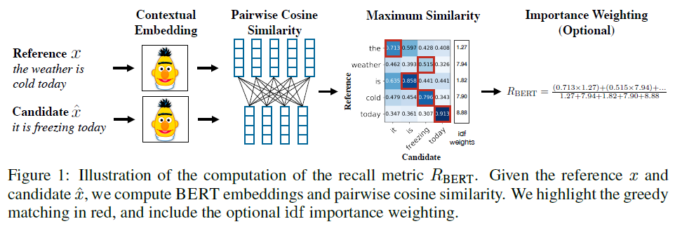
The score is rescaled from the range [-1, 1] to the range [0, 1] using the formula \(\hat R_{\mathrm{BERT}}=\frac{R_{\mathrm{BERT}}-b}{1-b}\), where \(b\) is the empirical lower bound of \(R_{\mathrm{BERT}}\) and computed by averaging \(R_{\mathrm{BERT}}\) of 1M pairs of random candidate-reference sentences from Common Crawl monolingual datasets. The same rescaling procedure is applied to \(P_{\mathrm{BERT}}\) and \(F_{\mathrm{BERT}}\). The rescaling does not affect the ranking ability and human correlation of BERTScore, and is solely to increase the score readability. BERTScore significantly outperforms BLEU (and several other earlier metrics) in terms of correlations with human judgement on machine translation and image captioning tasks. Overall, F1 \(F_{\mathrm{BERT}}\) performs better than \(R_{\mathrm{BERT}}\) and \(P_{\mathrm{BERT}}\). Computing BERTSore is relatively fast and suitable for using during validation and testing. An adversarial paraphrase classification task shows that BERTScore is more robust to challenging examples when compared to existing metrics.
Mover Score. Zhao et al. (2019)[39] introduce MoverScore that is similar to BERTScore in using pre-trained BERT contextual embeddings to encode tokens, but different from BERTScore by using Mover’s Distance to measure semantic distance between generated and reference responses. Let \(x=(\mathrm{x}_1,...,\mathrm{x}_m)\) and \(y=(\mathrm{y}_1,...,\mathrm{y}_l)\) be two sentences viewed as sequences of n-grams: \(x^n\) and \(y^n\) (e.g. \(x^1\) and \(x^2\) are sequences of unigrams and bigrams, respectively). Given a distance metric \(d\) between n-grams, the transportation cost matrix \(C\) is defined as having each element \(C_{ij}=d(\mathrm{x}_i^n,\mathrm{y}_j^n)\) representing the distance between the \(i\)-th n-gram of \(x^n\) and the \(j\)-th n-gram of \(y^n\). Let \(f_{x^n}\in\mathrm{\mathbb{R}}_{+}^{\vert x^n\vert}\) be a vector of weights, one weight for each n-gram of \(x^n\). The \(f_{x^n}\) is a distribution over \(x^n\), with \(f_{x^n}^{\top}\mathbf{1}=1\). The Word Mover’s Distance (WMD) between the two sequences of n-grams \(x^n\) and \(y^n\) with associated n-gram weights \(f_{x^n}\) and \(f_{y^n}\) is defined as: \(\mathrm{WMD}(x^n,y^n):=\min\limits_{F\in\mathrm{\mathbb{R}}^{\vert x^n\vert\times\vert y^n\vert}}\langle C,F\rangle\), such that \(F\mathbf{1}=f_{x^n}\) and \(F^{\top}\mathbf{1}=f_{y^n}\), where \(F\) is the transportation flow matrix with \(F_{ij}\) denoting the amount of flow traveling from the \(i\)-th n-gram \(\mathrm{x}_i^n\) in \(x^n\) to the \(j\)-th n-gram \(\mathrm{y}_j^n\) in \(y^n\). The \(\langle C,F\rangle\) denotes the sum of all matrix entries of the matrix \(C\odot F\), where \(\odot\) denotes element-wise multiplication. Then, \(\mathrm{WMD}(x^n,y^n)\) is the minimal transportation cost between \(x^n\) and \(y^n\), where n-grams are weighted by \(f_{x^n}\) and \(f_{y^n}\). The \(C_{ij}\) is computed by the Euclidean distance: \(d(\mathrm{x}_i^n,\mathrm{y}_j^n)=\Vert E(\mathrm{x}_i^n)-E(\mathrm{y}_j^n)\Vert_2\) where \(E\) is the embedding function which maps an n-gram to its vector representation. The embedding of an n-gram is computed as the weighted sum over its word embeddings, using Inverse Document Frequency (IDF) as weight. Given the \(i\)-th n-gram \(x_i^n=(\mathrm{x}_i,...\mathrm{x}_{i+n-1})\), its embedding is defined as: \(E(x_i^n)=\sum\limits_{k=i}^{i+n-1}\mathrm{idf}(\mathrm{x}_k)\cdot E(\mathrm{x}_k)\), where \(\mathrm{idf}(\mathrm{x}_k)\) is the IDF of word \(\mathrm{x}_k\) computed from all sentences in the corpus and \(E(\mathrm{x}_k)\) is its word embedding. The weight associated with \(x_i^n\) is defined as: \(f_{x_i^n}=\frac{1}{Z}\sum\limits_{k=i}^{i+n-1}\mathrm{idf}(\mathrm{x}_k)\), where \(Z\) a normalizing constant such that \(f_{x_i^n}^{\top}\mathbf{1}=1\).
When \(n\geq\) the length of a sentence, \(x^n\) contains only one n-gram that is the whole sentence. Then, \(\mathrm{WMD}(x^n,y^n)\) becomes Sentence Mover’s Distance (SMD), namely the distance between the two sentence embeddings, which is \(\mathrm{SMD}(x^n,y^n):=\Vert E(x_1^{l_x})-E(y_1^{l_y})\Vert\), where \(l_x\) and \(l_y\) are the lengths of the sentences.
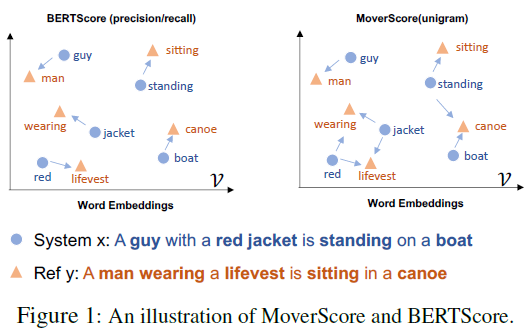
The primary difference between BERTScore and MoverScore is that the former can be viewed as one-to-one hard alignments of words in a sentence pair and the latter relies on many-to-one soft alignments, as illustrated in the Figure below. MoverScore can be viewed as finding the minimum effort to transform between two texts, by solving a constrained optimization problem. It can be proved that BERTScore (precision/recall) can be represented as a (non-optimized) Mover Distance \(\langle C,F\rangle\), where \(C\) is a transportation cost matrix based on BERT and \(F\) is a uniform transportation flow matrix.
Another difference is that BERTScore obtains embedding from single best layer, but MoverScore explores aggregating vectors produced by multiple layers. The aggregated embedding for the word \(x_i\) from \(L\) layers is denoted as \(E(x_i)=\phi((z_{i,l})_{l=1}^L)\), where \(z_{i,l}\in\mathrm{\mathbb{R}}^d\) denotes the \(d\)-dimensional vector produced by the \(l\)-th layer and \(\phi\) is an aggregation method that maps the \(L\) vectors to one final vector. One way of aggregation is the concatenation of power means. Let \(p\in\mathrm{\mathbb{R}}\cup\{\pm\infty\}\), the \(p\)-mean vector of \((z_{i,l})_{l=1}^L\) is: \(\mathrm{h}_i^{(p)}=(\frac{1}{L}\sum\limits_{l=1}^L z_{i,l}^p)^{1/p}\in\mathrm{\mathbb{R}}^d\) where exponentiation is applied elementwise. Then, several \(p\)-mean vectors of different \(p\) values are concatenated to form the final embedding vector: \(E(x_i)=\mathrm{h}_i^{(p_1)}\oplus ...\oplus\mathrm{h}_i^{(p_K)}\) where \(\oplus\) is vector concatenation and \(\{p_1,...,p_K\}\) are exponent values. In this paper, BERT embeddings are aggregated from the last five layers and \(K=3\) with \(p=\{1,\pm\infty\}\).
On machine translation, WMD-1/2+BERT+MNLI-finetuned+p-means outperforms not only BERTScore F1 but also supervised metric RUSE; also, word mover metrics outperforms the sentence mover. Lexical metrics can correctly assign lower scores to system translations of low quality, while they struggle to correctly assign higher scores to system translations of high quality. On the other hand, the word mover metric combining BERT can clearly distinguish system translations of both low and high qualities. On text summarization, WMD-1+BERT+MNLI+p-means outperforms BERTScore F1 but underperforms supervised metric \(S_{best}^3\). On Image Captioning, WMD-1+BERT+MNLI+p-means outperforms BERTScore-Recall but underperforms supervised metric LEIC. On task-oriented dialogue, all tested metrics, including WMD, perform poorly (Spearman correlation \(<0.3\)).
Learning-Based Metrics
Learning-based metrics can be subcategorized into four different approaches: (1) metrics learned from human-annotated scores, (2) metrics learned in unsupervised training, (3) pairwise-comparison-based rating systems, and (4) metrics derived from generation probabilities.
Metrics Learned from Annotated Scores
To train a dialog evaluation model that can predict scores like human-annotated scores requires sufficient amount of human-scored training dialog datasets. The scoring model is typically pre-trained as a language model or a dialog model and then fine-tuned with several thousand human-scored instances of dialogs for the scoring task. Three examples are covered here: (1) ADEM, pretrained as part of a dialog model using a latent variable hierarchical recurrent encoder decoder (VHRED) model; (2) BLEURT uses pretrained BERT language model; and (3) ENIGMA uses pretrained RoBERTa language model and formulates dialog evaluation as a model-free off-policy evaluation problem in reinforcement learning.
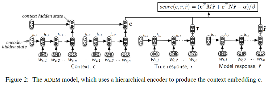
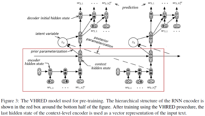
ADEM. Lowe et al. (2017)[53] introduced ADEM (Automatic Dialogue Evaluation Model) that learns to predict human-annotated appropriateness score of dialog responses. To learn from a full range of response qualities, a dataset of Twitter dialogs is used to collect 4 candidate responses per context from 4 different dialog models: (1) a TF-IDF retrieval-based model, (2) a Dual Encoder retrieval-based model, (3) a hierarchical recurrent encoder-decoder (HRED) generative model, and (4) human-generated responses, which are different from the reference responses from the Twitter Corpus. The responses are then judged by crowdsourced workers on overall appropriateness using scale of 1~5. The dataset contains 4,104 responses. ADEM aims to capture semantic similarity and to exploit both the context and the reference response to calculate its score for the model response. ADEM learns distributed representations of the context \(c\), reference response \(r\), and model response \(\hat r\), using a hierarchical RNN encoder, with LSTM units. The \(c,r,\hat r\) are first encoded into \(\mathrm{c},\mathrm{r},\mathrm{\hat r}\) vectors, respectively. Then, ADEM computes the score using a dot-product between the vector representations of \(c,r,\hat r\) in a linearly transformed space: \(score(c,r,\hat r)=(\mathrm{c}^{\top}M\mathrm{\hat r}+\mathrm{r}^{\top}N\mathrm{\hat r}-\alpha)/\beta\) where \(M,N\in\mathrm{\mathbb{R}}^{n\times n}\) are learned matrices initialized to the identity, and \(\alpha,\beta\) are scalar constants used to initialize the model’s predictions in the range [1, 5]. The matrices \(M\) and \(N\) can be interpreted as linear projections that map the model response \(\hat r\) into the space of contexts and reference responses, respectively. The parameters \(\theta=\{M,N\}\) of the model are trained to minimize the squared error between the model predictions and the human score, with L2-regularization: \(\mathcal{L}=\sum\limits_{i=1:K}[score(c_i,r_i,\hat r_i)-human_i]^2+\gamma\Vert\theta\Vert_2\) where \(\gamma\) is a scalar constant. The hierarchical RNN encoder in ADEM consists of two layers of RNNs, as illustrated in the Figure below. The lower-level is the utterance-level encoder that takes words from the dialogue as input and produces an output vector at the end (last hidden state) of each utterance, including contextual, reference response, and model response. The upper-level is the context-level encoder that takes contextual utterances representations as input and outputs the last hidden state as the vector representation of the context. The parameters of the hierarchical RNN encoder itself are not part of ADEM parameters and are not learned from the human-annotated scores.
The parameters of the hierarchical RNN encoder are pre-trained as part of a dialog model that attaches an additional decoder RNN on top of the encoder, takes the output of the encoder as the input of the decoder, and learns to predict the next utterance of a dialogue conditioned on the context. The dialog model is a latent variable hierarchical recurrent encoder decoder (VHRED) model that includes an additional turn-level stochastic latent variable, as illustrated in the Figure below. The latent variable is sampled from a multivariate Gaussian distribution and used along with the context vector as input to the decoder, which in turn generates the response word-by-word. The VHRED model is trained to maximize a lower-bound on the log-likelihood of generating the next response. The Gaussian latent variable allows modelling ambiguity and uncertainty in the dialog and helps generating more diverse responses. After training the VHRED, the last hidden state of the context-level encoder is used as the vector representations for \(\mathrm{c},\mathrm{r},\mathrm{\hat r}\).
ADEM correlates far better with human judgement than the word-overlap baselines: utterance-level Pearson correlations for (ADEM, tweet2vec embeddings, ROUGE, BLEU-2, METEOR) are (0.418, 0.141, 0.114, 0.081, 0.022), respectively.
BLEURT. Sellam et al. (2020)[44] introduced the BLEURT (Bilingual Evaluation Understudy with Representations from Transformers) metric that imitates human assessments by pre-training a fully learned metric on large amounts of synthetic data, before fine-tuning it on human ratings. Given a reference sentence \(x=(x_1,...,x_r)\) of length \(r\), where \(x_i\) denotes \(i\)-th token, a predicted sentence \(\tilde x=(\tilde x_1,...,\tilde x_p)\) of length \(p\), and a training dataset \(\{(x_n,\tilde x_n,y_n)\}_{n=1}^N\) of size \(N\) where \(y_n\in\mathrm{\mathbb{R}}\) is the human rating that indicates how good \(\tilde x_n\) is with respect to \(x_n\), the goal is to learn a function \(f:(x,\tilde x)\rightarrow y\) that predicts the human rating. Contextualized embeddings from BERT are used to represent tokens: \(v_{[\mathrm{CLS}]},v_{x_1},...,v_{x_r},v_{\tilde x_1},...,v_{\tilde x_p}=\mathrm{BERT}(x,\tilde x)\), where \(v_{[\mathrm{CLS}]}\) is the representation for the special token [CLS]. A linear layer is added on top of the [CLS] vector to predict the rating: \(\hat y=f(x,\tilde x)=W\tilde v_{[\mathrm{CLS}]}+b\), where \(W\) and \(b\) are the weight matrix and bias vector, respectively. Both the linear layer and the BERT parameters are fine-tuned on the supervised data which typically numbers in a few thousand examples. The regression loss is used: \(l_{\mathrm{supervised}}=\frac{1}{N}\sum_{n=1}^N\Vert y_i-\hat y\Vert^2\). However, fine-tuning BERT requires a sizable amount of IID data, which is less than ideal for a metric that should generalize to a variety of tasks and model drift.
Synthetic sentence pairs \((z,\tilde z)\) are generated by randomly perturbing 1.8 million segments \(z\) from Wikipedia to obtain about 6.5 million perturbations \(\tilde z\). Three techniques of perturbations are used. (1) Mask-filling with BERT: Masks are inserted at random positions or as contiguous sequences of masked tokens in Wikipedia sentences, then, the masks are filled with BERT language model. (2) Backtranslation: Paraphrases and perturbations are generated by translation from English to another language and then back to English with a translation model. (3) Dropping words: Some “pathological” examples are generated by randomly dropping words from the synthetic examples above. Each sentence pair \((z,\tilde z)\) is then augmented with a set of pre-training signals \(\{\tau_k\}\), where \(\tau_k\) is the target vector of pre-training task \(k\). Nine pre-training signals are used: three automatic metrics (\(\tau_{\mathrm{BLEU}}\),\(\tau_{\mathrm{ROUGE}}\),\(\tau_{\mathrm{BERTscore}}\)), four backtranslation likelihood metrics \(\tau_{\mathrm{en-fr},z\vert\tilde z}\), \(\tau_{\mathrm{en-fr},\tilde z\vert z}\), \(\tau_{\mathrm{en-de},z\vert\tilde z}\), \(\tau_{\mathrm{en-de},\tilde z\vert z}\), one textual entailment \(\tau_{\mathrm{entail}}\), and one backtranslation flag \(\tau_{\mathrm{backtran\_flag}}\). The \(\tau_{\mathrm{en-fr},\tilde z\vert z}\) is defined as \(\tau_{\mathrm{en-fr},\tilde z\vert z}=\frac{\log P(\tilde z\vert z)}{\vert\tilde z\vert}\), where \(P(\tilde z\vert z)=\sum\limits_{z_{\mathrm{fr}}}P_{\mathrm{fr\rightarrow en}}(\tilde z\vert z_{\mathrm{fr}})P_{\mathrm{en\rightarrow fr}}(z_{\mathrm{fr}}\vert z)\) and \(\vert\tilde z\vert\) is the number of tokens in \(\tilde z\). The summation \(\sum\limits_{z_{\mathrm{fr}}}\) is approximated by \(z_{\mathrm{fr}}^*=\mathrm{argmax}P_{\mathrm{en\rightarrow fr}}(z_{\mathrm{fr}}\vert z)\); thus, \(P(\tilde z\vert z)\approx P_{\mathrm{fr\rightarrow en}}(\tilde z\vert z_{\mathrm{fr}}^*)P_{\mathrm{en\rightarrow fr}}(z_{\mathrm{fr}}^*\vert z)\). By assuming that \(P_{\mathrm{en\rightarrow fr}}(z_{\mathrm{fr}}^*\vert z)\approx 1\), the backtranslation likelihood is reduced to \(P(\tilde z\vert z)\approx P_{\mathrm{fr\rightarrow en}}(\tilde z\vert z_{\mathrm{fr}}^*)\). The other three backtranslation likelihood metrics can be derived similarly. The \(\tau_{\mathrm{entail}}\) reports the probability of three labels: Entail, Contradict, and Neutral (from \(z\) to \(\tilde z\)), using BERT finetuned on an entailment dataset, MNLI. The signal \(\tau_{\mathrm{backtran\_flag}}\) is a Boolean that indicates whether the perturbation was generated with backtranslation or with mask-filling. The task-level losses are aggregated with a weighted sum. If \(\tau_k\) is a regression task, then \(l_2\) loss \(l_k=\Vert\tau_k-\hat\tau_k\Vert_2^2/\vert\tau_k\vert\) where \(\vert\tau_k\vert\) is the dimension of \(\tau_k\) and \(\hat\tau_k\) is computed by using a task-specific linear layer on top of the [CLS] embedding: \(\hat\tau_k=W_{\tau_k}\tilde v_{[\mathrm{CLS]}}+b_{\tau_k}\). If \(\tau_k\) is a classification task, a separate linear layer is used to predict a logit for each class \(c\): \(\hat\tau_{kc}=W_{\tau_{kc}}\tilde v_{[\mathrm{CLS]}}+b_{\tau_{kc}}\) and multiclass cross-entropy loss is used. The aggregate pre-training loss function is defined as: \(l_{\mathrm{pre-training}}=\frac{1}{M}\sum\limits_{m=1}^M\sum\limits_{k=1}^K\gamma_k l_k(\tau_k^m,\hat\tau_k^m)\), where \(\tau_k^m\) is the target vector for example \(m\), \(M\) is number of synthetic examples, and \(\gamma_k\) are hyperparameter weights obtained with grid search.
All BLEURT models are trained in three steps: (1) regular BERT pre-training, (2) pre-training on synthetic data (described above), and (3) fine-tuning on task-specific ratings (translation and/or data-to-text). BLEURT and BLEURT-base are based on BERT-large and BERT-base, respectively. For machine translation task, 2017 to 2019 WMT Metrics Shared Task to-English language pairs are used, which include several thousand pairs of sentences with human ratings in both training sets and test sets. The evaluation is to compare the correlation between the automatic metrics and the human ratings. BLEURT significantly outperforms MoverScore and BERTScore. Pre-training delivers consistent improvements, especially for BLEURT-base. Pre-training makes BLEURT significantly more robust to quality drifts. For data-to-text task, the WebNLG Challenge 2017 is used, which aims at generating natural language description of entities from sets of 1 to 5 RDF (Resource Description Framework) triples. The organizers released the human assessments for 4,677 sentence pairs. BLEURT was trained in three steps: first on synthetic data, then on WMT data, and finally on WebNLG data. When a record comes with several references, BLEURT is run on each reference and the highest value is reported. The more pre-trained BLEURT is, the quicker it adapts to the new task. BLEURT fine-tuned twice (first on synthetic data, then on WMT data) provides acceptable results on all tasks without task-specific training data. Ablation experiments show that pre-training signals of high quality (e.g., BERTscore, entailment, and the backtranslation scores) helps BLEURT, but signals that correlate less well with human judgment (e.g., BLEU and ROUGE) may harm the model.
ENIGMA. Jiang et al. (2021)[41] introduced ENIGMA (EvaluatiNg dIaloG systeMs Automatically) for estimating how a human would rate a dialog system by formulating automatic evaluation of dialogue systems as a model-free off-policy evaluation (OPE) problem in reinforcement learning, where the interactive process of a conversation is considered as a Markov decision process (MDP) and a human interlocutor is considered as the “environment”. A conversation is denoted as \(h=\{e_0,a_1,e_1,...,a_T\}\), where \(e_i\) and \(a_i\) are sentences generated by an environment \(\mathcal{E}\) (i.e., a human) and an agent \(\pi\) (i.e., a dialog system), respectively, and \(T\) is the number of turns in the conversation. Dialog can be naturally described as an MDP \(\mathcal{M}=\langle\mathcal{S},\mathcal{A},P,R,\mu_0\rangle\), where \(\mathcal{S}\), \(\mathcal{A}\), \(P\), \(R\), and \(\mu_0\) are states, actions, probabilities of transitions, rewards, and distribution of initial states, respectively. Specifically, at the \(t\)-th turn, state \(s_t\in\mathcal{S}\) captures the previous conversation history \(s_t=\{e_0,a_1,e_1,...,a_{t-1},e_{t-1}\}\). An action \(a_t\in\mathcal{A}\) is an agent’s response given \(s_t\). Conversation can then be represented by the last state and action, \(h=\{s_T,a_T\}\). An agent \(\pi\) is essentially a policy (i.e., a function) that maps \(\mathcal{S}\) to \(\mathcal{P}(\mathcal{A})\), where \(\mathcal{P}(\cdot)\) denotes the set of probability measures over the action space. A transition kernel \(P(\cdot\vert s_t,a_t)\) returns \(s_{t+1}\) as the state at turn \(t+1\), and an environment \(\mathcal{E}\) generates a reward \(r_t=R(s_t,a_t)\in[0,1]\). The \(s_{t+1}\) essentially concatenates \(s_t\) and \(a_t\) with \(e_t\), where \(e_t\) is a response from the environment at the \(t\)-th turn. The initial state \(s_1=\{e_0\}\) is randomly sampled from some distribution \(\mu_0\). The reward \(R\) measures language quality for open-domain chatbots and task completion scores for goal-oriented agents. Each conversation is only evaluated at the ending state, i.e., \(r_t=0\) for \(t<T\), which is the sparse reward setting.
Dialog evaluation can be viewed as the expected reward of the above MDP: \(\rho(\pi)=\mathrm{\mathbb{E}}_{h\sim\mu_0,\pi,\mathcal{E}}[R(s_T,a_T)]\), where conversation \(h=\{s_T,a_T\}\) is sampled from the initial distribution \(\mu_0\) and the interaction between \(\pi\) and \(\mathcal{E}\). When the environment (i.e., human) is accessible, \(\rho(\pi)\) can be directly estimated by interaction with the environment, which is known as on-policy evaluation. When access to the environment is limited or unavailable, \(\rho(\pi)\) can be estimated solely based on pre-collected tuples \(\{(s,a,r,s^{\prime})_i\}_{i=1}^N\) from behavior policies that are different from \(\pi\), which is known as off-policy evaluation (OPE). There are two types of OPE: (1) model-based OPE and (2) model-free OPE. The model-based OPE approach is to first directly learn an environment model (\(R\) and \(P\)) from experience data and then estimate \(\rho(\pi)\) by executing the policy within the learned environment, which corresponds to the so-called “self-play evaluation”. However, it is difficult to specify a proper model for a dialog environment due to the huge state and action spaces and model-based self-play evaluation of dialog systems often becomes unreliable. To avoid direct modeling of the environment, many model-free OPE methods have been proposed. Model-free OPE can be categorized into behavior-aware and behavior-agnostic methods. Behavior-aware methods rely on either knowing or accurately estimating the probabilistic model of behavior policies used for collecting the experience data, which is either unknown or difficult to estimate in practice. Behavior-agnostic methods do not require explicit knowledge or direct modeling of behavioral policies, and are more favorable when experience data is collected by multiple (potentially unknown) behavior policies.
ENIGMA is a model-free behavior-agnostic OPE method with three major ingredients: (1) pseudo-state padding for converting a dialog into an infinite-horizon MDP, (2) distribution-correction estimation with post-normalization for estimating the value of the target policy based on experience data, and (3) function approximation and representation learning with pre-trained language models. (1) Conversation sequences are padded with pseudo states to have a padded MDP with a fixed horizon length \(T_{max}\). A fixed horizon MDP is then converted into infinite horizon by augmentation (repeatedly concatenating the ending state of the fixed horizon MDP to its initial state). The augmented MDP with infinite horizon as “the augmented MDP”. The policy value of \(\pi\) for the augmented MDP can be defined as: \(\rho_A(\pi)=\lim_{N\rightarrow\infty}\mathrm{\mathbb{E}}_{(h_1,h_2,...,h_N)\sim\mu_0,\pi,\mathcal{E}}[\frac{1}{NT_{max}}\sum\limits_{i=1}^N\sum\limits_{t=1}^{T_{max}}R(s_t^{(i)},a_t^{(i)})]\), where \(h_i\)’s are padded conversations sampled from interactions between \(\pi\) and \(\mathcal{E}\). Since there is only one non-zero reward for every \(T_{max}\) steps, rewards in the augmented MDP are also sparse. It is proved that the augmented MDP has a unique stationary distribution and guarantees any policy \(\pi\) to have a finite policy value. Moreover, the policy value of \(\pi\) under the augmented MDP is proportional to its counterpart under the original MDP without augmentation. (2) Model-free behavior-agnostic DICE estimator is then applied to estimate \(\rho_A(\pi)\) based on pre-collected experience data \(\mathcal{D}=\{(s,a,r,s^{\prime})_i\}_{i=1}^N\) without interacting with \(\mathcal{E}\), where \((s,a)\sim d^{\mathcal{D}}\) are samples from some unknown distribution \(d^{\mathcal{D}}\). The notation \((s,a,r,s^{\prime})\sim d^{\mathcal{D}}\) is a shorthand for \((s,a)\sim d^{\mathcal{D}}\), \(r=R(s,a)\), \(s^{\prime}\sim P(\cdot\vert s,a)\), which simulates sampling from the dataset \(\mathcal{D}\). DICE decomposes \(\rho_A(\pi)\) into: \(\rho_A(\pi)=\mathrm{\mathbb{E}}_{(s,a,r)\sim d^{\mathcal{D}}}[\zeta(s,a)r]\), where \(\zeta(s,a):=d^{\pi}(s,a)/d^{\mathcal{D}}(s,a)\) is the distribution correction ratio. Then DICE estimates \(\zeta\) by solving the following regularized minimax optimization problem: \(\max\limits_{\zeta\geq 0}\min\limits_{\nu,\lambda}L_D(\zeta,\nu,\lambda)=\mathrm{\mathbb{E}}_{(s,a,r,s^{\prime})\sim d^{\mathcal{D}},a^{\prime}\sim\pi(s^{\prime})}[\zeta(s,a)\cdot(\nu(s^{\prime},a^{\prime})-\nu(s,a))]\) \(+\) \(\mathrm{\mathbb{E}}_{(s,a)\sim d^{\mathcal{D}}}[\lambda(\zeta(s.a)-1)]\) \(-\) \(\alpha_{\zeta}\cdot\mathrm{\mathbb{E}}_{(s,a)\sim d^{\mathcal{D}}}[f(\zeta(s.a))]\), where \(\nu(s,a)\)’s are auxiliary variables, \(f\) is a convex regularizer (e.g., \(f(x)=x^2\)), and \(\alpha_{\zeta}\) is a tuning parameter. The constraint \(\mathrm{\mathbb{E}}_{(s,a)\sim d^{\mathcal{D}}}\zeta(s.a)=1\) handled by Lagrange multipliers \(\lambda\) is enforced explicitly by a post-normalization step: \(\rho_n(\pi)=\sum_{(s,a,r)\sim d^{\mathcal{D}}}\zeta(s,a)r\Big/\sum_{(s,a)\sim d^{\mathcal{D}}}\zeta(s,a)\). The post-normalization step is crucial for DICE to attain good estimation accuracy in practice. (3) Pre-trained RoBERTa model is used to compute \(\zeta(s,a)\) and \(\nu(s,a)\). The encoder layers are kept, but the original mask language modeling heads are replaced by a two-layer fully connected network with a scalar output. The attention masks are modified to prevent tokens from attending future responses. RoBERTa-\(\zeta\) and RoBERTa-\(\nu\) denote \(\zeta(s,a)\) and \(\nu(s,a)\), respectively. RoBERTa-\(\zeta\) and RoBERTa-\(\nu\) share the same encoder, as illustrated below. RoBERTa-\(\zeta\) and RoBERTa-\(\nu\) are then used as the initial solution to solve the regularized minmax optimization problem above.
To test ENIGMA for evaluating goal-oriented dialog systems on a flight ticket booking task, transformer-based seller agent and transformer-based customer agent are used. The seller agent consists of four components for the encoder: ticket encoder, reservation encoder, dialog encoder, and task-specific heads (intent classification head and name classification head). The customer agent consists of two components for the encoder: intent encoder and reservation encoder. The AirDialog dataset is used for policy training (to train both seller and customer agents). Different proportions of the dataset and different hyperparameters are used to train 24 seller agents using behavior cloning. Twenty people interact with the 24 seller agents; each person interacts with a seller agent 5 times to collect experience data (based on the behavior policy of the seller agent) and give each interaction an evaluation score between 0 and 1 (i.e., true reward). The correlation between estimated reward and true reward are compared for ENIGMA, BLEU, Perplexity, and Self-Play Evaluation (SPE). Pearson Correlation of overall reward of ENIGMA, SPE, BLEU, and Perplexity are 0.8952, 0.4777, 0.2944, and 0.0460, respectively.
To test ENIGMA for evaluating open-domain chatbots, 29 pre-trained agents from [1] are used, which are based on 2-layer LSTM sequence-to-sequence model with attention. The ConvAI2 dataset[33] is used for policy training these agents using behavior cloning. The experience data provided by [1] are used, which contains 3,316 agent-human evaluation logs and 10 different language quality metrics (i.e., true rewards) for each log. The correlation between estimated reward and true reward are compared for ENIGMA, SPE, and 8 Hand-Crafted Dialog Features (HCDFs)[1]. Pearson Correlation of the average of the 10 language quality metrics of ENIGMA, the best of 8 HCDFs, and SPE are 0.9666, 0.6045, and 0.5907, respectively.
Metrics Learned in Unsupervised Training
Unsupervised training does not rely on human annotated scores as the training goal. Instead, it relies on automatically generated negative samples, either randomly or heuristically. It then learns to give higher scores to positive samples and lower scores to negative samples. Four examples are covered here: RUBER, BERT-RUBER, PONE, and GRADE.
RUBER. Tao et al. (2017)[54] introduced RUBER (Referenced metric and Unreferenced metric Blended Evaluation Routine) to combine an embedding-based referenced metric that measures the similarity between a generated reply and the ground truth and a neural network-based unreferenced metric that measures the relatedness between the generated reply and its query (i.e. context), as illustrated in the Figure below.
To measure the similarity between a generated reply \(\hat r\) and a ground truth \(r\) as the referenced metric, utterances are represented by choosing the maximum and minimum values in each dimension of constituent word embeddings and the closeness of a utterance pair is measured by the cosine score. Given \(w_1,w_2,...,w_n\) as the embeddings of words in an utterance, max-pooling summarizes the maximum value as \(v_{max}[i]=\max\{w_1[i],w_2[i],...,w_n[i]\}\) where \([\cdot]\) indexes a dimension of a vector. Similarly, min-pooling yields a vector \(v_{min}\). The two vectors are then concatenated to form the utterance representation \(v=[v_{max};v_{min}]\). The referenced metric \(s_R\) of the similarity between \(r\) and \(\hat r\) is computed by the cosine of the corresponding vectors \(v_r\) and \(v_{\hat r}\) : \(s_R(r,\hat r)=\cos(v_r,v_{\hat r})=\frac{v_r^{\top}v_{\hat r}}{\Vert v_r\Vert\cdot\Vert v_{\hat r}\Vert}\). This study uses 50-dimensional word2vec embeddings trained on Chinese online forum Douban.
To measure the relatedness between the generated reply \(\hat r\) and its query \(q\) as the unreferenced metric \(s_U(q,\hat r)\), a bidirectional recurrent neural network with gated recurrent units (Bi-GRU RNN) is used to encode an utterance along its word sequence into an embedding. The last states of both directions are concatenated as the utterance embedding. The vectors of query and generated reply are then concatenated with a “quadratic feature” \(q^{\top}\mathrm{M}r\) added in the middle, where \(\mathrm{M}\) is a parameter matrix, as illustrated in the Figure above. Finally, a multi-layer perceptron (MLP) predicts a scalar score as the unreferenced metric \(s_U\). The hidden layer of MLP uses tanh as the activation function, whereas the last (scalar) unit uses sigmoid function. To train the neural network, a negative sampling technique is used, where a negative reply \(r^-\) is randomly selected from the training set for a given ground truth query-reply pair. The score of a positive sample is expected to be larger than the score of a negative sample by at least a margin \(\Delta\). Thus, the training objective is to minimize \(J=\max\{0,\Delta-s_U(q,r)+s_U(q,r^-)\}\). The Chinese Douban training dataset consists of 1.45 million query-response pairs.
The above two metrics are combined by simple heuristics. The metrics are first normalized to the range of (0, 1) by \(\tilde s=\frac{s-\min(s^{\prime})}{\max(s^{\prime})-\min(s^{\prime})}\) where \(\min(s^{\prime})\) and \(\max(s^{\prime})\) refer to the minimum and maximum values, respectively, of a particular metric. Then, the normalized metrics \(\tilde s_R\) and \(\tilde s_U\) are combined to form the final RUBER score by heuristics including min, max, geometric averaging, or arithmetic averaging.
The RUBER metric (along with baselines) is evaluated on two prevailing dialog systems: (1) a feature-based retrieval-and-reranking system and (2) an RNN-based sequence-to-sequence (Seq2Seq) neural network with attention mechanism. Human rating on replies for meta-evaluation is done with 3-point scale: 0-bad, 1-borderline, 2-good. The correlation studies show that the referenced metric \(s_R\) is more correlated with human annotation than BLEU and ROUGE. The unreferenced metric \(s_U\) achieves even higher correlation than \(s_R\). RUBER-min, -geometric mean, and -arithmetic mean yield similar results. RUBER-max is worse than the other three. RUBER metric has near human correlation. On Seq2Seq with attention dialog model, the Pearson correlation of average inter-annotator and RUBER-min are 0.4708 and 0.4523, respectively.
BERT-RUBER. Ghazarian et al. (2019)[55] explored three ways of improving RUBER, particularly its unreferenced metric: (1) replacing static word2vec embeddings with contextualized BERT embeddings, (2) replacing Bi-RNN with simple pooling strategies to transform word embeddings into utterance embeddings, (3) replacing the ranking loss objective with a cross entropy loss objective, as illustrated in the Figure below.
The word2vec embeddings are 300 dimensional vectors trained on about 100 billion words of Google News Corpus. The BERT embeddings are 768 dimensional vectors pre-trained on Books Corpus and English Wikipedia with 3.3 billion words. For utterance encoding strategies, max pooling and mean pooling are compared with Bi-RNN with GRU units. The training objective of RUBER’s unreferenced metric is referred to as ranking loss objective, which uses a sigmoid function at the output of the last layer of the MLP. The cross-entropy loss in this study considers unreferenced score prediction as a binary classification problem with label “1” for the ground-truth query-response pair and label “0” for the negative sample. The output of softmax function in the last layer of the MLP classifier indicates the relatedness score for each pair of query and response. The Bi-GRU model of the unreferenced metric is trained with DailyDialog dataset. The dialog system used to evaluate the metrics is an attention-based Bi-LSTM sequence-to-sequence model that is also trained with DailyDialog dataset. To compute correlation between the metrics with human judgements, 300 pairs of query-generated response are annotated by 106 unique crowdsourced workers on the appropriateness of the generated response for the corresponding query on a scale of 1~5.
The 2 embedding approaches, 3 utterance representation approaches, and 2 objective functions result in 12 combinations. The correlations between unreferenced metrics and human judgments show that BERT-Max Pooling-Cross Entropy Loss combination (Pearson 0.55, Spearman 0.45) is substantially above other combinations, including RUBER’s word2vec-Bi-RNN-Ranking Loss (Pearson 0.28, Spearman 0.30). Contextualized embeddings in general outperform fixed embeddings when the other two variables are the same. Simple pooling of BERT embeddings, but bot word2vec embeddings, outperforms Bi-RNN encoding, with max pooling always better than mean pooling. Ranking loss generally performs better for models based on word2vec embeddings, while the best model with BERT embeddings is obtained by using cross-entropy loss.
PONE. Lan et al. (2020)[48] introduced the PONE (POsitive samples and valuable NEgative samples) metric that improves upon the RUBER and BERT-RUBER by adding more high-quality positive and negative samples for training the binary classifier scorer. Similar to the RUBER and BERT-RUBER, the scorer model consists of 3 stages: (1) the semantic representations of a context \(v_q\) and a response \(v_r\) are obtained by averaging their BERT-encoded word embeddings; (2) \(v_q\) and \(v_r\) are then concatenated together with a separator defined as \({v_q}^{\top}\mathrm{M}v_r\) where \(\mathrm{M}\) is a parameter matrix; (3) a multi-layer perception (MLP) uses the combined vector as input to predict a final metric score \(s\). The hidden layers of MLP use relu as the activation function, whereas the last unit uses sigmoid so that the score \(s\) is a real number between 0 and 1. The score can be interpreted as the probability of the given response being an appropriate response for the given context. The training objective is to minimize binary cross-entropy loss: \(J=\frac{1}{K}\sum\limits_i^K-y_i\cdot\log\bar{y_i}-(1-y_i)\cdot\log(1-\bar{y_i})\) where \(K\) is the size of the whole generated dataset, \(y_i\) is the label of the \(i\)-th example, \(\bar{y_i}\) is the label of \(i\)-th example generated by the scorer.
In typical negative sampling datasets, for a given context, there is only one positive response and many randomly sampled negative responses that are often low-quality and not informative for learning. Therefore, the decision boundary learned from such dataset can be far from the real boundary, as illustrated in the Figure below. To reduce the difference between the real decision boundary and the generated decision boundary, PONY uses a weighted negative sampler to select valuable negative samples instead of random samples and a positive data generator to provide lots of effective positive samples which alleviates the imbalanced data distribution. In addition, a label filter algorithm is used for reducing noise in augmented data.
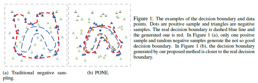
The weighted negative sampler first randomly extracts \(h\) candidate negative samples \(\{n_i\}_{i=1}^h\) from the whole datasets. Then, semantic similarities are computed between the ground-truth \(r\) and the candidate negative samples \(\{n_i\}_{i=1}^h\) using cosine similarity \(\cos(v_r,v_{n_i})=\frac{v_r^{\top}v_{n_i}}{\Vert v_r\Vert\ \Vert v_{n_i}\Vert}\), where \(v_r\) and \(v_{n_i}\) are average BERT-encoded word embeddings of \(r\) and \(n_i\), respectively. Finally, the cosine similarities are converted to selective probabilities by applying the softmax with a temperature factor \(t\): \(p(v_r,v_{n_i})=\frac{e^{\cos(v_r,v_{n_i})/t}}{\sum_i^h e^{\cos(v_r,v_{n_i})/t}}\). The performance is best when the \(t\) is between 0.05 and 0.1. For the positive data generator, two data augmentation methods are tried: (1) Easy Data Augmentation (EDA) techniques, including synonym replacement, random insertion, random swap, and random deletion, which tend to generate samples containing lots of noise; (2) generative dialog model Seq2Seq with beam search. The augmented positive samples for the context \(q_i\) is denoted as \(\{r_{ij}\}_{j=1}^k\), where \(k\) is the size. The performance is best when the \(k\) is 5. To reduce the effect of noisy (false positive) samples, a novel iterative algorithm, named label filter, is applied to assign the real label for each augmented sample. First, the scorer is pre-trained with the positive and negative samples. Then, the pre-trained scorer is used to generate pseudo labels for positive samples generated by the positive data generator. Then, the scorer is fine-tuned by the negative samples and the augmented positive samples (with pseudo labels). Finally, the process is iterated until the pseudo labels of the augmented samples no longer change.
In both single-turn and multi-turn dialog evaluations, PONE significantly outperforms BERT-RUBER and BERTScore.
GRADE. Huang et al. (2020)[45] introduced GRADE (Graph-enhanced Representation for Automatic Dialogue Evaluation) to evaluate dialog coherence by explicitly modeling topic transition dynamics using graph reasoning and incorporating them into utterance-level contextualized representations, based on the idea that the topics inside a coherent dialog are close to each other in the commonsense graph. GRADE is trained in an unsupervised manner with data automatically generated by a negative sampling strategy considering both lexical and semantic aspects. Given a dialog context \(c=\{c_1,...,c_m\}\) and a response \(r=\{r_1,...,r_n\}\), where each \(c_k\) is a token in the context and each \(r_k\) is a token in the response, the goal is to learn a function \(f:(c,r)\rightarrow s\) that predicts the coherence score \(s\). As illustrated in the Figure below, GRADE predicts a coherence score \(s\) between \(c\) and \(r\) in three steps: (1) producing the utterance-level contextualized representation \(v_c\); (2) generating the topic-level graph representation \(v_g\); (3) predicting the coherence score \(s\) based on \(v_c\) and \(v_g\). In step (1), BERT is used to encode the \(c\) and \(r\). The pooled output feature of BERT is taken as the utterance-level contextualized representation \(v_c\): \(v_c=BERT(c,r)\).
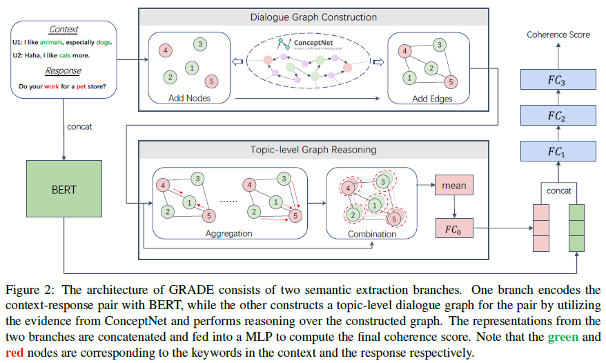
In step (2), there are two stages: dialog graph construction and topic-level graph reasoning. In the first stage, a topic-level dialog graph \(G=(V,E)\) is constructed based on \(c\) and \(r\), where \(V\) is a set of topic nodes and \(E\) is a set of edges between topics. The nodes are topic keywords extracted by a rule-based keyword extractor that combines both TF-IDF and Part-Of-Speech features. The keywords in \(c\) are the context-topic nodes of \(G\), \(V_c=\{t_1,t_2,...,t_p\}\), while the keywords in \(r\) are the response-topic nodes of \(G\), \(V_r=\{t_{p+1},t_{p+2},...,t_{p+q}\}\), where \(p\) and \(q\) are the numbers of keywords in the context \(c\) and the response \(r\), respectively. Therefore, \(V=V_c\cup V_r\). Then, ConceptNet is used to obtain node representations. Each topic node \(t_i\) is aligned to the corresponding node in ConceptNet and first initialized as \(h_i=CN(t_i)\in\mathrm{\mathbb{R}}^d\), \(i\in[1,p+q]\), where \(h_i\) is the initial representation of the node \(t_i\), \(CN\) is the ConceptNet Numberbatch embeddings, and \(d\) is the dimension of each node representation. To capture topic relations, \(h_i\) is updated with the representations of its k-hop neighboring representations: \(h_{\bar{\mathcal{N}}_i^k}=\frac{1}{\vert\bar{\mathcal{N}}_i^k\vert}\sum\limits_{t_j\in\bar{\mathcal{N}}_i^k}CN(t_j)\), \(\bar h_i=h_i+\sum\limits_{k=1}^K(W_k h_{\bar{\mathcal{N}}_i^k}+b)\), where \(K\) is the maximum number of hops taken into account and is set as 2, \(\bar{\mathcal{N}}_i^k\) is the \(k^{th}\) hop neighboring nodes of \(t_i\) in the ConceptNet graph, \(W_k\) and \(b\) are the weight matrix and bias vector, respectively. The edges only exist between each context-topic node \(V_c^i\) and each response-topic node \(V_r^j\), because the goal is to predict a coherence score of a response based on a context. \(G\) is considered as a weighted undirected graph, the weight of each edge is assigned heuristically using the hop information in the ConceptNet commonsense graph, named as hop-attention weight. Let the weighted adjacency matrix of \(G\) as \(A\), then the hop-attention weight of the edge between the nodes \(t_i\) and \(t_j\) (i.e., \(A[i][j]\)) is determined by: \(A[i][j]=\frac{1}{\#hops(V_c^i,V_r^j)}\), where \(\#hops(\cdot)\) indicates the shortest path between \(V_c^i\) and \(V_r^j\) over the ConceptNet graph. DropEdge technique is used to prevent over-smoothing by randomly deactivating a certain number of edges at each training step. The adjacency matrix \(A\) is normalized: \(\bar A=(D+I)^{-1/2}(A+I)(D+I)^{-1/2}\), where \(\bar A\) is the augmented normalized adjacency matrix, \(D\) is the corresponding degree matrix of \(A\), and \(I\) is the identity matrix. In the second stage: the topic transition dynamics is modeled by reasoning over the constructed topic-level graph \(G\) via two steps: aggregation and combination. In the aggregation step, the graph attention network is applied to aggregate neighboring information of each node \(t_i\). The aggregated representation \(z_i^{(l)}\) at the layer \(l\) for the node \(t_i\) is formulated as follows: \(z_i^{(l)}=\sum\limits_{j\in\mathcal{N}_i}\alpha_{ij}\mathrm{W}_lh_j^{(l)}\), \(\alpha_{ij}=\frac{\exp(e_{ij})}{\sum_{n\in\mathcal{N}_i}\exp(e_{in})}\), \(e_{ij}=\bar A[i][j]\ast\rho(a_l^{\top}[\mathrm{W}_lh_i^{(l)}\Vert\mathrm{W}_lh_j^{(l)}])\), where \(h_i^{(0)}=\bar h_i\), \(\mathcal{N}_i\) is the neighboring nodes of \(t_i\) in the dialog graph \(G\), \(\mathrm{W}_l\in\mathrm{\mathbb{R}}^{d\times d}\) and \(a_l\in\mathrm{\mathbb{R}}^{2d}\) are learnable parameters, \(\alpha_{ij}\) is the attention coefficient, \(\rho\) is LeakyReLU, and \(\cdot^{\top}\) represents transposition. The \(e_{ij}\) scales the attention coefficient \(\alpha_{ij}\) with the augmented normalized adjacency matrix \(\bar A\), so that the network will pay more attention to the nodes that are closer to \(t_i\) in the ConceptNet graph during the aggregation. In the combination step, the aggregated representation \(z_i^{(l)}\) is combined with the \(i^{th}\) node representation \(h_i^{(l)}\) to get the updated node representation \(h_i^{(l+1)}\): \(h_i^{(l+1)}=ELU(\mathrm{V}_lh_i^{(l)}+z_i^{(l)})\), where \(\mathrm{V}_l\in\mathrm{\mathbb{R}}^{d\times d}\) is the weight matrix to transform \(h_i^{(l)}\), and \(ELU\) represents an exponential linear unit. Finally, the topic-level graph representation \(v_g\) is obtained by: \(v_g=FC_0(mean(\{h_i^{L}\vert i\in[1,p+q]\}))\), where \(h_i^{(L)}\) is the \(i^{th}\) node representation at the last layer, \(mean\) represents mean pooling, and \(FC_0\) is a fully-connected layer with an \(ELU\) activation.
In step (3), the contextualized representation \(v_c\) and the graph representation \(v_g\) are concatenated together and fed into a multi-layer perceptron (MLP) to transform the high-dimensional representation into the coherence score \(s\), a real number: \(s=FC_3(FC_2(FC_1([v_c;v_g])))\), where \(FC_1\), \(FC_2\), and \(FC_3\) are three different fully-connected layers whose activation functions are \(ELU\), \(ELU\), and sigmoid, respectively.
GRADE is trained in an unsupervised manner. Given a dataset \(D=\{(c_i,r_i,\bar r_i)\vert i\in[1,N]\}\), where \(c_i\) and \(r_i\) are a ground-truth context-response pair and \(\bar r_i\) is a false response for the context \(c_i\) selected by using negative sampling, GRADE is trained to predict a higher score for each ground-truth response \(r_i\) than its corresponding false response \(\bar r_i\) by minimizing the following margin ranking loss: \(\mathcal{L}=\frac{1}{N}\sum\limits_{i=1}^Nmax(0,\bar s_i-s_i+m)\), where \(N\) is the size of the dataset, \(m\) is a margin value set as 0.1, \(s_i\) and \(\bar s_i\) are the coherence scores of \(r_i\) and \(\bar r_i\), respectively, in the \(i^{th}\) example. Negative samples are generated by two sampling methods: lexical sampling and embedding-based sampling. For lexical sampling, Lucene is used to retrieve utterances that are related to the ground-truth response \(r\) from the training set, and select the middle one in the retrieved utterances as the false response \(\bar r\). For embedding-based sampling, BERT-encoded utterance embeddings are used for cosine similarity-based selection. In 1000 randomly sampled utterances, the top-5 with the highest cosine similarity with the ground-truth response \(r\) are selected, one of which is then randomly selected to be the false response \(\bar r\). On DailyDialog dataset for dialog models using Transformer-Ranker and Transformer-Generator, GRADE obtains the highest correlations with human judgements in average (0.294), significantly above BLEURT (0.284), BERT-RUBER (0.184), BERTScore (0.168), and ADEM (0.128). GRADE can easily adapt to other unseen datasets without any re-training and obtain more stable and higher correlations with human judgements (average correlation 0.579 on ConvAI2 and 0.298 on EmpatheticDialogues) than the baseline metrics. Ablation studies show that (1) random sampling causes 6.6% performance drop compared to negative sampling, (2) removing the graph branch or the k-hop neighboring representations decrease performance, and (3) the best performance is from adopting the 2-hop neighboring representations and 10 nodes in each of the 1st and 2nd hop.
GRADE adopts the ranking loss that only requires good responses to be ranked higher than bad responses, a relatively loose constraint compared with the absolute scoring that humans do. Therefore, GRADE may deviate from the human scoring criterion and fail to quantify the dialogue responses accurately, and that the human correlation results fluctuate over different runs.
Pairwise-Comparison-Based Rating Systems
This approach is an automatic counterpart of the pairwise human evaluations.
Comparative Evaluator. To compare the quality of texts generated by NLG models, Zhou and Xu (2020)[49] introduced a text pair relation classifier that is trained to classify whether the first text is better (\(>\)), worse (\(<\)), or indistinguishable (\(\approx\)) when compared with the second text. A skill rating system is then used to perform model-level evaluation based on the sample-level evaluation results provided by the pairwise comparison model. A pre-trained BERT model is used for the comparative evaluator, as illustrated by the Figure below. To ensure that the paired texts, sample A and sample B, are comparable, they are based on the same context.
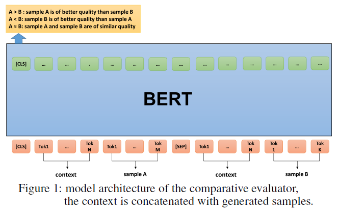
Three types of training examples are used to fine-tune the pre-trained BERT model: (1) strong supervision examples, (2) weak supervision examples, and (3) human-annotated examples. (1) In strong supervision, human written responses \(s_+\in S_+\) are designated to have higher quality than model-generated responses \(s_-\in S_-\). Thus, (\(s_+,s_-\)) has the label “better (\(>\))”; (\(s_-,s_+\)) has the label “worse (\(<\))”; and (\(s_+^i,s_+^j\)) and (\(s_-^i,s_-^j\)) have the label “indistinguishable (\(\approx\))”. When constructing a (\(s_-^i,s_-^j\)), \(s_-^i\) and \(s_-^j\) are sampled from the same checkpoint of the same model. For a training set with \(n\) real samples and \(n\) generated samples, \((_2^{2n})\) pairwise training examples can be constructed for the comparative evaluator. Because \((_2^{2n})=2\times(_2^{n})+n^2\), the pairwise approach introduces more informative learning signals than the standard real/fake binary discriminative evaluator. (2) In weak supervision, samples generated by later checkpoint are designated to have higher quality than samples generated by earlier version of the same model. Sufficient improvement in later checkpoints is ensured by setting the minimal margin between two selected checkpoints to be 10% of the total training iteration and not selecting two “almost converged” checkpoints. In addition, sample pairs with larger margin are used during initial training stage and the margin is decreased gradually to capture smaller quality differences. (3) When human preference annotation is available, the comparative evaluator is additionally fine-tuned with human annotations. The comparative evaluator is trained with maximum likelihood estimation (MLE) objective: \(L=-\mathrm{\mathbb{E}}_{(x_1,x_2)\sim\mathcal{X}}[\log D_{\phi}^{Q(x_1,x_2)}(x_1,x_2)]\) where \(\mathcal{X}\) is the set of pairwise training examples, \(Q(x_1,x_2)\in\{>,<,\approx\}\) is the true label for the pair \((x_1,x_2)\), \(D_{\phi}^q(x_1,x_2)\) is the probability of the comparative evaluator’s prediction being \(q\) (\(q\in\{>,<,\approx\}\)) for the pair \((x_1,x_2)\).
In two-player games, such as chess and tennis, a skill rating system ranks players by observing the records of wins and losses of multiple players and inferring the value of a latent, unobserved skill variable for each player that explains the records of wins and losses. In this study, a skill rating system is adopted for model-level evaluation of NLG models. Taking the trained comparative evaluator as the “playground” and NLG models as “players”, the “two-player game” is played by sampling one output sample from each NLG model conditioning on the same input and the game outcome is decided by the comparative evaluator. The skill rating system, Glicko-2[50], is used in this study, which considers each player’s skill rating as a Gaussian distribution, with a mean and standard deviation, representing the current state of the evidence about the “true” skill rating. A simple rule is used to handle a “tie”: the skill level of one player is increased/decreased by a fraction (e.g. 0.1) of the changes for wins/loses if the player draws with another player with higher/lower skill rating. In this study, the skill rating is performed by randomly sampling from two compared models, simulating a “game” between two selected models by sampling one sample from each model and comparing them with the comparative evaluator, and then updating the skill rating of selected models according to the outcome. This procedure is performed iteratively until convergence, which is defined as the order of skill ratings of compared models keeps the same after each model is selected at least 50 times.
For meta-evaluation, 20 human annotators provide 5-point Likert scores on overall sample quality. Inter-annotator agreement of direct scoring and pairwise comparison are evaluated. For the pairwise comparison, 20 generated samples are paired with 4 other generated samples and are scored to 1~5 based on how many times (can be 0~4) they are considered to be better. The inter-annotator agreement scores are \(\kappa=0.53\) and \(\kappa=0.76\) for direct scoring and pairwise comparison, respectively, suggesting that pairwise comparison is more accurate than direct scoring. At both sample-level and model-level, the comparative evaluator correlates far better with human judgement than BLEU, Perplexity, Adversarial Evaluator, and ADEM.
The comparative evaluator is also used for selecting hyperparameters and early-stopping during model training. For choosing hyperparameters, skill rating is performed among all models trained with 5 randomly sampled hyperparameter choices in a predefined range. For early-stopping, pairwise comparisons are performed \(n\) (e.g. 1000) times between the samples generated by the latest checkpoint and the previous \(k\) (e.g. 2) checkpoints and stop training when the wining rate of latest checkpoint keeps being smaller than its losing rate for 5 iterations. Human evaluation is then employed to identify the best choice. The comparative evaluator substantially outperforms BLEU, Perplexity, Adversarial Evaluator, and ADEM in both hyperparameter tuning and early-stopping checkpoint selecting. Ablation studies show the relative importance of the components of the comparative evaluator as: comparison > tie option > fine-tuning with human annotation > pre-trained BERT > fine-tuning with strong supervision > fine-tuning with weak supervision.
Metrics Derived from Generation Probabilities
In this approach, the quality score of a dialog response is formulated as a function of the generation probability of the response given the context. Four examples are covered here: Context Coherence, FED, USR, and Perception Score.
Context Coherence. Pang et al. (2020)[8] use language modeling to naturally capture the coherence of the response to the dialogue context (or query). Pre-trained GPT-2 is fine-tuned using the next sentence prediction task on the dialogue datase of DailyDialog. Given token sets of query \(q\) and response \(r\) as \(\{q_t:t=1,...,T_q\}\) and \(\{r_t:t=1,...,T_r\}\) and the fine-tuned GPT-2 as \(P\), the context coherence is defined as the log-likelihood of the response conditional on the the query normalized by the length of the response length: \(c_{raw}(r\vert q)=\frac{1}{T_r}\log\frac{P(q,r)}{P(q)}=\frac{1}{T_r}\sum\limits_t^{T_r}\log P(r_t\vert r_{<t},q)\). \(c_{raw}(r\vert q)\) is negative and unbounded at lower end. To avoid extreme values, the \(c_{raw}(r\vert q)\) is normalized to have values in the range from 0 to 1 using the equation: \(c(r\vert q)=-\frac{\max(c_{5th},c_{raw}(r\vert q))-c_{5th}}{c_{5th}}\), where \(c_{5th}\) is the 5th percentile of \(c_{raw}(r\vert q)\). The language model based coherence metric shows high correlation with human evaluation (Pearson’s \(r=0.67\), Spearman’s \(\rho=0.76\)) and the correlations are close to inter-rater correlations (Pearson’s \(r=0.61\), Spearman’s \(\rho=0.57\)).
FED. Mehri and Eskenazi (2020)[40] introduced the FED (Fine-grained Evaluation of Dialog) metric that uses pre-trained DialoGPT model to evaluate multifaceted qualities of generated responses by the log-likelihood of generating aspect-specific follow-up utterances. The DialoGPT is trained on GPT-2 architecture using 147M conversations from Reddit; thus, it is assumed to have implicitly captured some notion of dialog quality. Although it does not need reference response, it requires manually written aspect-specific follow-up responses to the system responses to be evaluated. It is assumed that user response to a given system utterance may implicitly or explicitly provide feedback for the system. For each fine-grained dialog qualities, a set of positive follow-up utterances, \(p\), and a set of negative follow-up utterances, \(n\), are constructed. Given a dialog context \(c\), a system response \(r\), and a function \(\mathcal{D}\) that computes the log-likelihood of DialoGPT generating a particular response, the predicted quality score for a turn-level dialogue quality is defined as: \(\sum\limits_{i=1}^{\vert p\vert}\mathcal{D}(c+r,p_i)-\sum\limits_{i=1}^{\vert n\vert}\mathcal{D}(c+r,n_i)\). To predict scores for dialogue-level qualities, the \(r\) is removed from the equation. For each quality aspect, 0~4 positive utterances and 1~4 negative utterances are hand-written and minimally tuned on a small subset (10 conversations) of the FED dataset. The overall impression scores are calculated as an average of the scores for either the turn-level or dialog-level qualities. Most of the turn-level qualities are scored using only the last system response as context. For relevant, correct, and dialogue-level metrics, the entire conversation is used as context. The pre-trained DialoGPT models can be either medium (345M) or large (762M), and either fine-tuned from GPT-2 or trained from scratch. The Spearman correlation was measured between the predicted quality scores and the mean of the annotated scores. The best overall correlation score is 0.209 and 0.443 for turn-level and dialogue-level, respectively, which is slightly better than prior work. The FED metric works better for some dialog qualities than others. For example, it is more likely that DialoGPT learns to measure qualities like interesting and engaging, than understandable and consistent. FED metric attains moderate correlation with human judgements across all the systems. The FED metric is not a replacement for human evaluation, but a mean of measuring dialog quality for the purposes of validation and model tuning.
USR. Mehri and Eskenazi (2020)[47] introduced the USR (UnSupervised and Reference-free) evaluation metric that is composed of multiple sub-metrics of specific dialog qualities in a configurable manner. USR leverages pre-trained RoBERTa to measure 5 sub-metrics for 5 qualities of dialog: Understandable, Natural (human-like), Maintains Context (coherent), Interesting, and Uses Knowledge (factual consistent), which are combined to form the USR score. Two types of models are used to measure the sub-metrics: Masked Language Modelling (MLM) for evaluating Understandable, Natural and Dialog Retrieval (DR) for evaluating Maintains Context, Interesting, and Uses Knowledge.
The MLM metric uses a RoBERTa model fine-tuned on the corpus being evaluated (either Topical-Chat or PersonaChat) to estimate the likelihood of a response. When the Topical-Chat training set is used for the fine-tuning, only the dialogs, not the facts, are used. RoBERTa uses both past and future context to predict a probability distribution for a masked word. The input sequence to MLM is a concatenation of a dialog context, \(c\), and a response, \(r\). One word at a time, each word in \(r\) is masked and its log-likelihood is computed. Given the masked log-likelihood for the \(i\)-th word of \(r\) as \(l_i\), the value of the metric is then computed to be \(-\sum_i^{\vert r\vert}l_i\). For DR metrics, the above fine-tuned RoBERTa model is further fine-tuned for the retrieval task using the Ubuntu dialog corpus. The model is trained given a context \(x\), a response \(r\), and a binary label \(y\) indicating whether \(r\) is the true response or randomly sampled. The context \(x\) may consist of the dialog history and the fact, denoted \(c\), or just the fact, denoted \(f\). Two different versions of the dialog retrieval (DR) metric are trained, with different values of \(x\) (\(x=c\) or \(x=f\)). The DR metric score is defined to be the probability \(P(y = 1\vert x,r)\) a given DR metric model produces. The DR metric is trained to distinguish between a ground-truth response (\(y=1\)) and a randomly sampled response (\(y=0\)). The automatic sub-metrics are then combined into one measure of overall quality using a regression model that is trained to map the five human-annotated sub-metrics to the human-annotated overall quality score, as described earlier. The best sub-metrics for each dialog quality are used as input for the regression model of the USR metric. While the best performing sub-metrics are not consistent across the two datasets, the USR metric nonetheless exhibits strong results. As shown by the correlations with human evaluation scores, USR strongly outperforms both word-overlap and embedding-based metrics (including BERTScore-base) across all five dialog qualities on both Topical-Chat and PersonaChat datasets, at both turn-level and system-level.
Perception Score. Gu et al. (2020)[42] introduced Perception Score that measures the overall quality of an open-ended generative model by assigning a single holistic score based on the distribution difference between the generations and the references. The evaluation process of Perception Score contains three steps: (1) A Perception Model will learn to assign a sample level Perception Score based on a generated sentence’s overall quality; (2) The uncertainty is calculated for the sample level Perception Score; and (3) Sample level scores and uncertainties are aggregated to get the system-level Perception Score for the generation model.
(1) Perception Score aims at comparing generations \(G=\langle\hat x_1,...,\hat x_n\rangle\) with corresponding references \(R=\langle x_1,...,x_n\rangle\), where \(\hat x_i\) and \(x_i\) denote the generation and reference, respectively, of the \(i\)-th sample in the dataset. Perception Score is defined as a function \(\delta\) that perceives realness of the generation. Since standard of realness changes across NLG tasks, Perception Score should be learned to fit various NLG tasks. The realness is defined by aggregating the distances between every pair of samples: \(\delta_{\theta}=\mathrm{argmax}_{\theta}\mathrm{\mathbb{E}}_{\hat x\sim\mathrm{\mathbb{P}}_G,x\sim\mathrm{\mathbb{P}}_R}[\delta_{\theta}(\hat x,x)]\). To get a more comprehensive semantic representation, context \(c_i\) is incorporated into \(G\) and \(R\) to obtain \(G^+=\langle\{c_1,\hat x_1\},...,\{c_n,\hat x_n\}\rangle\) and \(R^+=\langle\{c_1,x_1\},...,\{c_n,x_n\}\rangle\). The goal of Perception Score is to compute a reasonable and efficient approximation of Earth Mover’s Distance (EMD): \(W(\mathrm{\mathbb{P}}_{G^+},\mathrm{\mathbb{P}}_{R^+})=\inf\limits_{\gamma\in\prod(\mathrm{\mathbb{P}}_{G^+},\mathrm{\mathbb{P}}_{R^+})}\mathrm{\mathbb{E}}_{(x,\hat x)\sim\gamma}[\Vert x-\hat x\Vert]\), where \(\prod(\mathrm{\mathbb{P}}_{G^+},\mathrm{\mathbb{P}}_{R^+})\) denotes the set of all joints distributions. \(\gamma\) indicates how much “mass” must be transported from \(\hat x\) to \(x\) in order to transform the distribution \(\mathrm{\mathbb{P}}_{G^+}\) to the distribution \(\mathrm{\mathbb{P}}_{R^+}\). The formula can be converted to the supremum over the 1-Lipschitz functions[43]: \(W(\mathrm{\mathbb{P}}_{G^+},\mathrm{\mathbb{P}}_{R^+})=\sup\limits_{\vert f\vert_L\leq 1}\mathrm{\mathbb{E}}_{x\sim\mathrm{\mathbb{P}}_{R^+}}[f(x)]-\mathrm{\mathbb{E}}_{\hat x\sim\mathrm{\mathbb{P}}_{G^+}}[f(\hat x)]\), which is equivalent to optimize the following problem \(W(\mathrm{\mathbb{P}}_{G^+},\mathrm{\mathbb{P}}_{R^+})=\max\limits_{\theta}\mathrm{\mathbb{E}}_{\hat x\sim\mathrm{\mathbb{P}}_{G^+},x\sim\mathrm{\mathbb{P}}_{R^+}}[f_{\theta}(x)-f_{\theta}(\hat x)]\) with a gradient penalty loss to fulfill the Lipschitz constrain \(L_{GP}=\mathrm{\mathbb{E}}_{\hat x\sim\mathrm{\mathbb{P}}_{G^+},x\sim\mathrm{\mathbb{P}}_{R^+}}[(\Vert\nabla_{\hat x,x}D(\hat x,x)\Vert_2-1)^2]\). To avoid divergence, the maximum earth-mover distance is bounded to be 1 by normalizing the output. \(f_{\theta}(\hat x)=\frac{e^{l_1(T(\hat x))}}{e^{l_1(T(\hat x))}+e^{l_1(T(x))}}=P_{generated}\) and \(f_{\theta}(x)=\frac{e^{l_1(T(x))}}{e^{l_1(T(\hat x))}+e^{l_1(T(x))}}=P_{reference}\), where \(l_1\) is linear forward layers, and \(T(x)\) and \(T(\hat x)\) denote the output of the Perception model of reference sample and generated sample, respectively, as illustrated in the Figure below. Optimizing \(P_{reference}\) is equivalent to optimizing EMD distance. The Perception Model learns the difference of a generated sentence and its corresponding reference sentence in the training set, and evaluate the generation model quality on the test set.
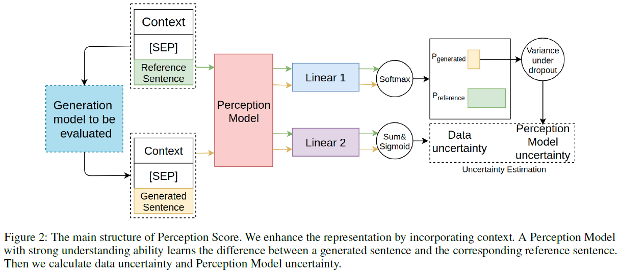
(2) Sample-level uncertainties are used as weights during score aggregation. Both data uncertainty and model uncertainty are used in Perception Score evaluation. For model uncertainty \(m\), the variance of the prediction under different dropout settings are used: \(m=1-\mathrm{Var}(P_{generated})\). For data uncertainty, an additional fully-connected layers \(l_2\) is used to get the confidence degree \(c\) for the Perception Score and a sigmoid function is used to constrain uncertainty between 0 and 1: \(c=sigmoid(l_2(T(\hat x)+T(x)))\), where \(\hat x\in\mathrm{\mathbb{P}}_{G^+}\) and \(x\in\mathrm{\mathbb{P}}_{R^+}\). Then the optimization objective is adjusted by interpolating between the original Perception Score and the data uncertainty: \(p^{\prime}=c\cdot P_{reference}+(1-c)y\), where \(y\) is the target distribution. \(p^{\prime}\) is optimized: \(\mathcal{L}_t=-\sum\limits_{i=1}^M\log(p_i^{\prime})\). An extra regularizer is used to prevent the network from minimizing the loss by always choosing data uncertainty \(c\) as 0, \(\mathcal{L}_c=-\log(c)\). Final uncertainty for each sample is a simple addition of data uncertainty and model uncertainty. Final loss is a weighted sum of the data uncertainty loss and Perception Score loss: \(\mathcal{L}=\mathcal{L}_t+\lambda\mathcal{L}_c+\beta L_{GP}\), where \(\lambda\) and \(\beta\) are hyperparameters.
(3) During test time, the system-level Perception Score \(P_{sys}\) for \(G\) is computed as weighted sum of \(P_{generated}\): \(P_{sys}=\sum\limits_{i=1}^n w_i\times P_{generated}^i\), where the weight \(w\) is calculated by model uncertainty \(m\) and data uncertainty \(c\) as \(w_i=\frac{c_i+m_i}{\sum_{k=1}^n c_k+m_k}\). Higher \(P_{sys}\) means higher generation system quality. When \(P_{sys}\) is around 0.5, the Perception Model considers the generated senrtences and the references having similar quality.
Two versions of Perception Model are used: RoBERTa-base and RoBERTa-large. Three conditional generation tasks and two unconditional generation tasks are evaluated. Perception Score outperforms, in terms of correlation with human judgement, all other tested metrics by a large margin in all 5 tasks. For example, in ROCStories task, where the goal is to generate an open-ended story ending for a four-sentence short context, the correlation is 0.692, 0.529, 0.331, 0.328, and 0.282 by Perception Score-large, BLEURT-large, Comparator Evaluator, MoverScore-large, and BERTScore-large, respectively. Ablation studies show that data uncertainty contributes more to the evaluation performance than the model uncertainty, and incorporating context is necessary when Perception Score is used in conditional generation tasks.
Codes
- ParAI provides integration with Amazon Mechanical Turk for human evaluation of chatbots.
- Pyro’s source code and documentation & examples
- Human Evaluation Datasheet
- NLP Power Analysis
- Maximum Match Size of Bitext Grid
- Hugging Face Metrics code and description
- spaCy code and documentation
- LanguageTool code and documentation
- BERTScore
- MoverScore
- FED code and FED Dataset
- USR code and Annotated Datasets
- ENIGMA code, Transformer model for AirDialog, and Experience data for OPE on ConvAI2
- BLEURT
- GRADE
- ConceptNet Numberbatch embeddings
- Apache Lucene, a high-performing full-featured text search engine library
- \(Q^2\)
- Chinese Word Vectors 中文字向量
- PONE
- pyglicko2, a Python implemenation of Glicko-2
- Predictive Engagement
- ADEM
References
[1] See, A., Roller, S., Kiela, D., and Weston, J. (2019) What makes a good conversation? How controllable attributes affect human judgments. arXiv preprint arXiv:1902.08654
[2] Smith, E. M., Williamson, M., Shuster, K., Weston, J., and Boureau, Y-L. (2020) Can you put it all together: Evaluating conversational agents’ ability to blend skills. arXiv preprint arXiv:2004.08449
[3] Zhang, Y., Sun, S., Galley, M., Chen, Y., Brockett, C., Gao, X., Gao, J., Liu, J., and Dolan, B. (2019) DIALOGPT : Large-Scale Generative Pre-training for Conversational Response Generation. arXiv preprint arXiv:1911.00536
[4] Adiwardana, D., Luong, M., So, D., Hall, J., Fiedel, N., Thoppilan, R., Yang, Z., Kulshreshtha, A., Nemade, G., Lu, Y., and Le, Q. (2020) Towards a Human-like Open-Domain Chatbot. arXiv preprint arXiv:2001.09977
[5] Smith, E. M., Gonzalez-Rico, D., Dinan, E., and Boureau, Y-L. (2020) Controlling Style in Generated Dialogue. arXiv preprint arXiv:2009.10855
[6] Bao, S., He, H., Wang, F., Wu, H., Wang, H., Wu, W., Guo, Z., Liu, Z., Xu, X. (2020) PLATO-2: Towards Building an Open-Domain Chatbot via Curriculum Learning. arXiv preprint arXiv:2006.16779
[7] Shuster, K., Poff, S., Chen, M., Kiela, D., Weston, J. (2021) Retrieval Augmentation Reduces Hallucination in Conversation. arXiv preprint arXiv:2104.07567
[8] Pang, B., Nijkamp, E., Han, W., Zhou, L., Liu, Y., and Tu, K. (2020) Towards Holistic and Automatic Evaluation of Open-Domain Dialogue Generation. In: Proceedings of the 58th Annual Meeting of the Association for Computational Linguistics, 3619–3629.
[9] Krippendorff, K. (2011) Computing Krippendorff’s Alpha-Reliability.
[10] Celikyilmaz, A., Clark, E., and Gao, J. (2020) Evaluation of Text Generation: A Survey. arXiv preprint arXiv:2006.14799
[11] Tay, L. and Ng, V. (2018) Ideal Point Modeling of Non-cognitive Constructs: Review and Recommendations for Research. Frontiers in Psychology, 9:2423.
[12] Dalal, D. K., Carter, N. T., and Lake, C. J. (2014) Middle Response Scale Options are Inappropriate for Ideal Point Scales. Journal of Business and Psychology, 29(3), 463–478.
[13] Kulikov, I., Miller, A. H., Cho, K., and Weston, J. (2018) Importance of Search and Evaluation Strategies in Neural Dialogue Modeling. arXiv preprint arXiv:1811.00907
[14] Bingham, E., Chen, J. P., Jankowiak, M., Obermeyer, F., Pradhan, N., Karaletsos, T., Singh, R., Szerlip, P., Horsfall, P., and Goodman, N. D. (2018) Pyro: Deep Universal Probabilistic Programming. arXiv preprint arXiv:1810.09538
[15] Hoffman, M. D. and Gelman, A. (2011) The no-u-turn sampler: adaptively setting path lengths in hamiltonian monte carlo. arXiv preprint arXiv:1111.4246
[16] Venkatesh, A., Khatri, C., Ram, A., Guo, F., Gabriel, R., Nagar, A., Prasad, R., Cheng, M., Hedayatnia, B., Metallinou, A., Goel, R., Yang, S., and Raju, A. (2018) On Evaluating and Comparing Open Domain Dialog Systems. arXiv preprint arXiv:1801.03625
[17] Howcroft, D. M., Belz, A., Clinciu, M., Gkatzia, D., Hasan, S. A., Mahamood, S., Mille, S., van Miltenburg, E., Santhanam, S., and Rieser, V. (2020) Twenty Years of Confusion in Human Evaluation: NLG Needs Evaluation Sheets and Standardised Definitions. In: Proceedings of the 13th International Conference on Natural Language Generation, pages 169–182.
[18] Belz, A., Mille, S., and Howcroft, D. M. (2020) Disentangling the Properties of Human Evaluation Methods: A Classification System to Support Comparability, Meta-Evaluation and Reproducibility Testing. In: Proceedings of the 13th International Conference on Natural Language Generation, pages 183–194.
[19] Shimorina, A. and Belz, A. (2021) The Human Evaluation Datasheet 1.0: A Template for Recording Details of Human Evaluation Experiments in NLP. arXiv preprint arXiv:2103.09710
[20] Card, D., Henderson, P., Khandelwal, U., Jia, R., Mahowald, K., and Jurafsky, D. (2020) With Little Power Comes Great Responsibility. In: Proceedings of the 2020 Conference on Empirical Methods in Natural Language Processing, pages 9263–9274.
[21] Liu, C.-W., Lowe, R., Serban, I. V., Noseworthy, M., Charlin, L., and Pineau, J. (2016) How NOT To Evaluate Your Dialogue System: An Empirical Study of Unsupervised Evaluation Metrics for Dialogue Response Generation. arXiv preprint arXiv:1603.08023
[22] Papineni, K., Roukos, S., Ward, T., and Zhu, W.-J. (2002) Bleu: a method for automatic evaluation of machine translation. In: Proceedings of the 40th Annual Meeting of the Association for Computational Linguistics. Association for Computational Linguistics, pages 311-318.
[23] Melamed, I.D., Green, R., and Turian, J. P. (2003) Precision and Recall of Machine Translation.
[24] Doddington, G. (2002) Automatic Evaluation of Machine Translation Quality Using N-gram Co-Occurrence Statistics. In: Proceedings of the second international conference on Human Language Technology Research, pages 138-145.
[25] Lin, C.-Y. (2004) ROUGE: A Package for Automatic Evaluation of Summaries. In: Proceedings of the Workshop on Text Summarization Branches Out, pages 74-81.
[26] Banerjee, S. and Lavie, A. (2005) METEOR: An Automatic Metric for MT Evaluation with Improved Correlation with Human Judgments. In: Proceedings of the ACL Workshop on Intrinsic and Extrinsic Evaluation Measures for Machine Translation and/or Summarization, pages 65-72.
[27] Galley, M., Brockett, C., Sordoni, A., Ji, Y., Auli, M., Quirk, C., Mitchell, M., Gao, J., and Dolan, B. (2015) \(\Delta\)BLEU: A Discriminative Metric for Generation Tasks with Intrinsically Diverse Targets. arXiv preprint arXiv:1506.06863
[28] Dusek, O., Novikova, J., and Rieser, V. (2020) Evaluating the state-of-the-art of End-to-End Natural Language Generation: The E2E NLG challenge. In: Computer Speech & Language, 59: pages 123-156.
[29] Gehrmann, S., Adewumi, T., Aggarwal, K., Ammanamanchi, P. S., Anuoluwapo, A., et al. (2021) The GEM Benchmark: Natural Language Generation, its Evaluation and Metrics. arXiv preprint arXiv:2102.01672
[30] Zhu, Y., Lu, S., Zheng, L., Guo, J., Zhang, W., Wang, J., and Yu, Y. (2018) Texygen: A Benchmarking Platform for Text Generation Models. arXiv preprint arXiv:1802.01886
[31] Dinan, E., Roller, S., Shuster, K., Fan, A., Auli, M., and Weston, J. (2018) Wizard of Wikipedia: Knowledge-powered Conversational Agents. arXiv preprint arXiv:1811.01241
[32] Zhou, X., Li, L., Dong, D., Liu, Y., Chen, Y., Zhao, W. X., Yu, D., and Wu, H. (2018) Multi-Turn Response Selection for Chatbots with Deep Attention Matching Network. In: Proceedings of the 56th Annual Meeting of the Association for Computational Linguistics (Long Papers), pages 1118–1127
[33] Dinan, E., Logacheva, V., Malykh, V., Miller, A., Shuster, K., Urbanek, J., Kiela, D., Szlam, A., et al. (2019) The Second Conversational Intelligence Challenge (ConvAI2). arXiv preprint arXiv:1902.00098
[34] Serban, I. V., Sordoni, A., Bengio, Y., Courville, A., and Pineau, J. (2015) Building End-To-End Dialogue Systems Using Generative Hierarchical Neural Network Models. arXiv preprint arXiv:1507.04808
[35] Conley, T., St. Clair, J., and Kalita, J. (2021) Improving Computer Generated Dialog with Auxiliary Loss Functions and Custom Evaluation Metrics. arXiv preprint arXiv:2106.02516
[36] Berlot-Attwell, I. and Rudzicz, F. (2021) On the Use of Linguistic Features for the Evaluation of Generative Dialogue Systems. arXiv preprint arXiv:2104.06335
[37] Guo, F., Metallinou, A., Khatri, C., Raju, A., Venkatesh, A., and Ram, A. (2018) Topic-based Evaluation for Conversational Bots. arXiv preprint arXiv:1801.03622
[38] Zhang, T., Kishore, V., Wu, F., Weinberger, K. Q., and Artzi, Y. (2019) BERTScore: Evaluating Text Generation with BERT. arXiv preprint arXiv:1904.09675
[39] Zhao, W., Peyrard, M., Liu, F., Gao, Y., Meyer, C. M., and Eger, S. (2019) MoverScore: Text Generation Evaluating with Contextualized Embeddings and Earth Mover Distance. arXiv preprint arXiv:1909.02622
[40] Mehri, S. and Eskenazi, M. (2020) Unsupervised Evaluation of Interactive Dialog with DialoGPT. arXiv preprint arXiv:2006.12719
[41] Jiang, H., Dai, B., Yang, M., Zhao, T., and Wei, W. (2021) Towards Automatic Evaluation of Dialog Systems: A Model-Free Off-Policy Evaluation Approach. arXiv preprint arXiv:2102.10242
[42] Gu, J., Wu, Q., and Yu, Z. (2020) Perception Score: A Learned Metric for Open-ended Text Generation Evaluation. arXiv preprint arXiv:2008.03082
[43] Arjovsky, M., Chintala, S., and Bottou, L. (2017) Wasserstein GAN. arXiv preprint arXiv:1701.07875
[44] Sellam, T., Das, D., and Parikh, A. P. (2020) BLEURT: Learning Robust Metrics for Text Generation. In: Proceedings of the 58th Annual Meeting of the Association for Computational Linguistics, pages 7881–7892
[45] Huang, L., Ye, Z., Qin, J., Lin, L., and Liang X. (2020) GRADE: Automatic Graph-Enhanced Coherence Metric for Evaluating Open-Domain Dialogue Systems. arXiv preprint arXiv:2010.03994
[46] Honovich, O., Choshen, L., Aharoni, R., Neeman, E., Szpektor, I., and Abend, O. (2021) \(Q^2\): Evaluating Factual Consistency in Knowledge-Grounded Dialogues via Question Generation and Question Answering. arXiv preprint arXiv:2104.08202
[47] Mehri, S. and Eskenazi, M. (2020) USR: An Unsupervised and Reference Free Evaluation Metric for Dialog Generation. arXiv preprint arXiv:2005.00456
[48] Lan, T., Mao, X.-L., Wei, W., Gao, X., and Huang, H. (2020) PONE: A Novel Automatic Evaluation Metric for Open-Domain Generative Dialogue Systems. arXiv preprint arXiv:2004.02399
[49] Zhou, W. and Xu, K. (2020) Learning to Compare for Better Training and Evaluation of Open Domain Natural Language Generation Models. arXiv preprint arXiv:2002.05058
[50] Glickman, M. E. (2013) Example of the Glicko-2 system. Mark Glickman’s World.
[51] Fleiss, J. L. (1971) Measuring nominal scale agreement among many raters. Psychological Bulletin, Vol. 76, No. 5 pp. 378–382
[52] Ghazarian, S., Weischedel, R., Galstyan, A., and Peng, N. (2019) Predictive Engagement: An Efficient Metric for Automatic Evaluation of Open-Domain Dialogue Systems. arXiv preprint arXiv:1911.01456
[53] Lowe, R., Noseworthy, M., Serban, I. V., A.-Gontier, N., Bengio, Y., and Pineau, J. (2017) Towards an Automatic Turing Test: Learning to Evaluate Dialogue Responses. arXiv preprint arXiv:1708.07149
[54] Tao, C., Mou, L., Zhao, D., and Yan, R. (2017) RUBER: An Unsupervised Method for Automatic Evaluation of Open-Domain Dialog Systems. arXiv preprint arXiv:1701.03079
[55] Ghazarian, S., Wei, J. T.-Z., Galstyan, A., and Peng, N. (2019) Better Automatic Evaluation of Open-Domain Dialogue Systems with Contextualized Embeddings. arXiv preprint arXiv:1904.10635